03: Species interactions
Fallert, S. and Cabral, J.S.
Source:vignettes/species_interactions.Rmd
species_interactions.RmdTo make the example from the “Introduction / Get started” vignette more interesting, we can introduce more processes around the interaction between the two species.
First we will generate the same setup.
sim <- create_simulation(create_example_landscape())
sim$add_species(name = "species_1")
sim$add_species(name = "species_2")

sim$add_traits(
    species = c("species_1", "species_2"),
    population_level = TRUE,
    abundance = 500,
    climate_suitability = 1,
    reproduction_rate = 0.3,
    carrying_capacity = 1000
)
sim$add_traits(
    species = c("species_1", "species_2"),
    population_level = FALSE,
    dispersal_kernel = calculate_dispersal_kernel(
        max_dispersal_dist = 3,
        kfun = negative_exponential_function,
        mean_dispersal_dist = 1
    )
)
sim$add_traits(
    species = "species_1",
    population_level = FALSE,
    max_temperature = 300,
    optimal_temperature = 288,
    min_temperature = 280,
    max_precipitation = 1000,
    optimal_precipitation = 700,
    min_precipitation = 200
)
sim$add_traits(
    species = "species_2",
    population_level = FALSE,
    max_temperature = 290,
    optimal_temperature = 285,
    min_temperature = 270,
    max_precipitation = 1000,
    optimal_precipitation = 500,
    min_precipitation = 0
)
sim$add_process(
    species = c("species_1", "species_2"),
    process_name = "calculate_suitability",
    process_fun = function() {
        self$traits$climate_suitability <-
            calculate_suitability(
                self$traits$max_temperature,
                self$traits$optimal_temperature,
                self$traits$min_temperature,
                self$sim$environment$current$temperature
            ) *
            calculate_suitability(
                self$traits$max_precipitation,
                self$traits$optimal_precipitation,
                self$traits$min_precipitation,
                self$sim$environment$current$precipitation
            )
    },
    execution_priority = 1
)
sim$add_process(
    species = c("species_1", "species_2"),
    process_name = "reproduction",
    process_fun = function() {
        self$traits$carrying_capacity <-
            self$traits$carrying_capacity *
            self$traits$climate_suitability

        self$traits$reproduction_rate <-
            self$traits$reproduction_rate *
            self$sim$environment$current$habitat

        self$traits$abundance <-
            ricker_reproduction_model(
                self$traits$abundance,
                self$traits$reproduction_rate,
                self$traits$carrying_capacity
            )
    },
    execution_priority = 2
)
sim$add_process(
    species = c("species_1", "species_2"),
    process_name = "dispersal_process",
    process_fun = function() {
        self$traits[["abundance"]] <- dispersal(
            abundance = self$traits[["abundance"]],
            dispersal_kernel = self$traits[["dispersal_kernel"]])
    },
    execution_priority = 3
)
Competition
We’ll start by adding a process that simulates competition between the two species. This process will reduce the carrying capacity of a habitat cell based on the abundance of the other species. For simplicity, we’ll assume asymmetric competition, with species 1 being the superior competitor. Therefore we’ll only reduce the carrying capacity of species 2 based on the abundance of species 1.
sim$add_process(
    species = "species_2",
    process_name = "competition",
    process_fun = function() {
        self$traits$carrying_capacity <-
            self$traits$carrying_capacity - self$sim$species_1$traits$abundance

        self$traits$carrying_capacity[self$traits$carrying_capacity < 0] <- 0
    },
    execution_priority = 4
)
Note that this happens after the reproduction process, so the carrying capacity will be reduced for the next time step, not the current one. One could change this by changing the execution priority of the competition process.
sim$begin()
plot_cols <- hcl.colors(100, "Purple-Yellow", rev = TRUE)
plot(sim, "species_1", "abundance", main = "Sp: 1 abundance", col = plot_cols)
plot(sim, "species_2", "abundance", main = "Sp: 2 abundance", col = plot_cols)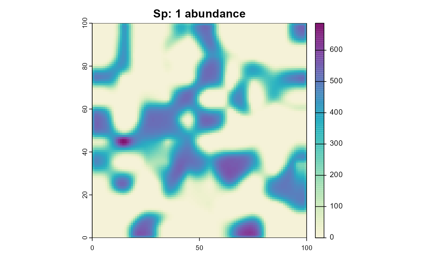

As you can see, species 2 is only able to survive in habitat that is unsuitable for species 1.
Throphic interactions
We can also add a process that simulates trophic interactions in the form of predation. Assuming that species 2 is a predator and species 1 is its prey, this means that species 2 will reduce the abundance of species 1, but can only occur in the same areas as species 1. We’ll again use a similar setup as before, with slightly adjusted values:
sim <- create_simulation(create_example_landscape())
sim$add_species(name = "species_1")
sim$add_species(name = "species_2")

sim$add_traits(
    species = "species_1",
    population_level = TRUE,
    abundance = 10000,
    climate_suitability = 1,
    reproduction_rate = 0.5,
    carrying_capacity = 10000
)
sim$add_traits(
    species = "species_2",
    population_level = TRUE,
    abundance = 500,
    climate_suitability = 1,
    reproduction_rate = 0.3,
    carrying_capacity = 1000
)
sim$add_traits(
    species = c("species_1", "species_2"),
    population_level = FALSE,
    dispersal_kernel = calculate_dispersal_kernel(
        max_dispersal_dist = 3,
        kfun = negative_exponential_function,
        mean_dispersal_dist = 1
    )
)
sim$add_traits(
    species = "species_1",
    population_level = FALSE,
    max_temperature = 300,
    optimal_temperature = 290,
    min_temperature = 270,
    max_precipitation = 1000,
    optimal_precipitation = 800,
    min_precipitation = 0
)
sim$add_traits(
    species = "species_2",
    population_level = FALSE,
    max_temperature = 300,
    optimal_temperature = 270,
    min_temperature = 260,
    max_precipitation = 1000,
    optimal_precipitation = 300,
    min_precipitation = 0
)
sim$add_process(
    species = c("species_1", "species_2"),
    process_name = "calculate_suitability",
    process_fun = function() {
        self$traits$climate_suitability <-
            calculate_suitability(
                self$traits$max_temperature,
                self$traits$optimal_temperature,
                self$traits$min_temperature,
                self$sim$environment$current$temperature
            ) *
            calculate_suitability(
                self$traits$max_precipitation,
                self$traits$optimal_precipitation,
                self$traits$min_precipitation,
                self$sim$environment$current$precipitation
            )
    },
    execution_priority = 1
)
sim$add_process(
    species = c("species_1", "species_2"),
    process_name = "reproduction",
    process_fun = function() {
        self$traits$carrying_capacity <-
            self$traits$carrying_capacity *
            self$traits$climate_suitability

        self$traits$reproduction_rate <-
            self$traits$reproduction_rate *
            self$sim$environment$current$habitat

        self$traits$abundance <-
            ricker_reproduction_model(
                self$traits$abundance,
                self$traits$reproduction_rate,
                self$traits$carrying_capacity
            )
    },
    execution_priority = 2
)
sim$add_process(
    species = c("species_1", "species_2"),
    process_name = "dispersal_process",
    process_fun = function() {
        self$traits[["abundance"]] <- dispersal(
            abundance = self$traits[["abundance"]],
            dispersal_kernel = self$traits[["dispersal_kernel"]])
    },
    execution_priority = 3
)
But now with a process that simulates predation. Note that the predation effectiveness is dependent on the climate suitability of the predator.
sim$add_globals(trophic_conversion_factor = 0.5)
sim$add_process(
    species = "species_2",
    process_name = "predation",
    process_fun = function() {
        self$traits$abundance <-
            self$sim$species_1$traits$abundance *
            self$traits$climate_suitability *
            self$sim$globals$trophic_conversion_factor

        self$sim$species_1$traits$abundance <-
            self$sim$species_1$traits$abundance -
            self$sim$species_1$traits$abundance *
            self$traits$climate_suitability
    },
    execution_priority = 4
)
sim$begin()
plot_cols <- hcl.colors(100, "Purple-Yellow", rev = TRUE)
plot(sim, "species_1", "abundance", main = "Sp: 1 abundance", col = plot_cols)
plot(sim, "species_2", "abundance", main = "Sp: 2 abundance", col = plot_cols)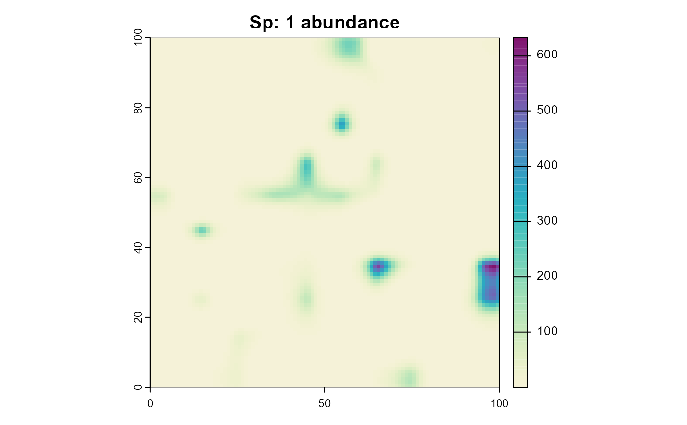
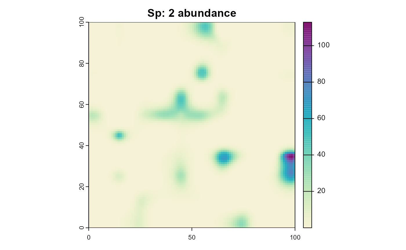
Note how species 2 occupies the same areas as species 1 despite having a completely different climatic niche. Reminder:
species_1
max_temperature = 300
optimal_temperature = 290
min_temperature = 270
max_precipitation = 1000
optimal_precipitation = 800
min_precipitation = 0
species_2
max_temperature = 300
optimal_temperature = 270
min_temperature = 260
max_precipitation = 1000
optimal_precipitation = 300
min_precipitation = 0