01: Introduction to metaRange

In general, metaRange is a framework to build a variety of different process based species distribution models. The package is build around an simulation object that manages the simulation state. This simulation object contains an environment that holds and manages all the environmental factors that may influence the simulation (as raster data) and it can contain one or more species that are simulated in the environment. Each species has two main characteristics: traits which can be (somewhat arbitrary) pieces of data that describe the species and processes which are functions that describe how the species interacts with itself, time, climate and other species. During each time step of the simulation, the processes are executed in a user defined order and can access and modify the species traits.

While the models built with metaRange can be quite variable in their structure, they are all based on population dynamics. This means that in most cases a trait will not be a singular number but a matrix that has the same size as the raster data in the environment, where each value represents the trait value for one population in the corresponding grid cell of the of the environment. Based on this, most processes will describe population (and meta population) dynamics and not individual based mechanisms. Figure 1 shows an example of some of the different envionmental factors, species traits and processes that could be included in a simulation.

Figure 1: Example of some of the different envionmental factors, species traits and processes that could be included in a simulation.

A more technical overview of the different components of a simulation and how they interact with each other is shown in Figure 2. While the environment has a temporal dimension (i.e. the different time steps, see Fig.1), the traits (or the global variables of the simulation) have no temporal property. They represent the state of the species (or of the simulation respectivly) in one (the current) time step. When a process is executed within a time step, it can access this current state of the simulation and modify it, which results in changing traits over the course of the simulation. Each process can be assigned a priority, that is used by the process priority queue to determine in which order the processes are executed within one time step.

Figure 2: Overview of the different components of a simulation and how they interact with each other. Note that the number of species & processes per species is not limited, but only two are shown for simplicity.

Setting up a simulation

Following is a simple example of how to set up a simulation with metaRange. To start, we need to load the package and its dependencies.

library(metaRange)
#> metaRange version: 0.0.0.9000
library(terra)
#> terra 1.7.55

Loading the landscape

The first step when setting up a simulation is the loading of the environment in which the simulation will take place. In the real world, this data can be obtained from a variety of sources, and may include for example different climate variables, land cover or elevation.

The simulations expects this data as an SpatRasterDataset (SDS) which is a collection of different raster files that all share the same extent and resolution. Each sub-dataset in this SDS represents one environmental variable and each layer represents one time step of the simulation. In other words, metaRange doesn’t simulate the environmental conditions itself, but expects the user to provide the environmental data for each time step.

To create such an dataset one can use the function terra::sds(). One important note: Since the layer represent the condition in one time step, all the raster files that go into the SDS need to have the same number of layer (i.e. the desired number of time steps the simulation should have). After the SDS is created, the individual subdatasets should be named, since this is how the simulation will refer to them.

To simplify this introduction, we use a randomly generated landscape consisting of temperature, precipitation and habitat quality data, with 10 time steps (layer) that are all the same (i.e. no environmental change). If you are interested, you can find the code to generate this landscape at the end of this vignette, but otherwise it’s enough to know that throughout this tutorial create_example_landscape() does create such a landscape.

landscape <- create_example_landscape()
landscape
#> class       : SpatRasterDataset 
#> subdatasets : 3 
#> dimensions  : 100, 100 (nrow, ncol)
#> nlyr        : 10, 10, 10 
#> resolution  : 1, 1  (x, y)
#> extent      : 0, 100, 0, 100  (xmin, xmax, ymin, ymax)
#> coord. ref. :  
#> source(s)   : memory 
#> names       : temperature, precipitation, habitat


terra::plot(
    landscape$temperature[[1]],
    col = hcl.colors(100, "Geyser"),
    main = "Temperature [K]")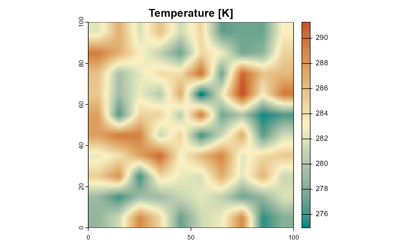

Figure 3: The temperature of the example landscape. Only the first layer of 10 identical ones is shown.

terra::plot(
    landscape$precipitation[[1]],
    col = hcl.colors(100, "GnBu", rev = TRUE),
    main = "Precipitation [mm]")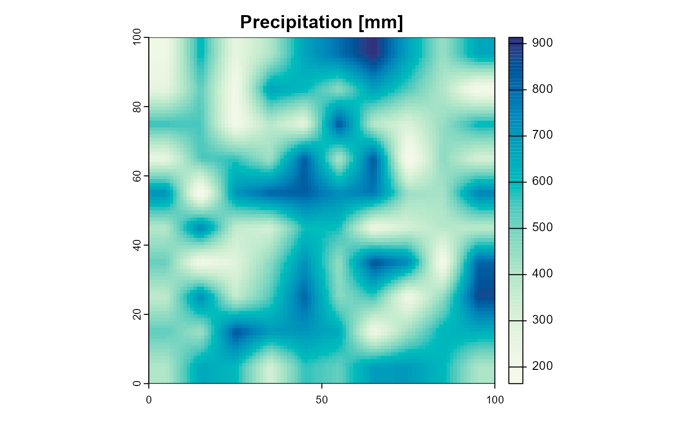

Figure 4: The precipitation of the example landscape. Only the first layer of 10 identical ones is shown.

terra::plot(
    landscape$habitat[[1]],
    main = "Habitat quality [0-1]")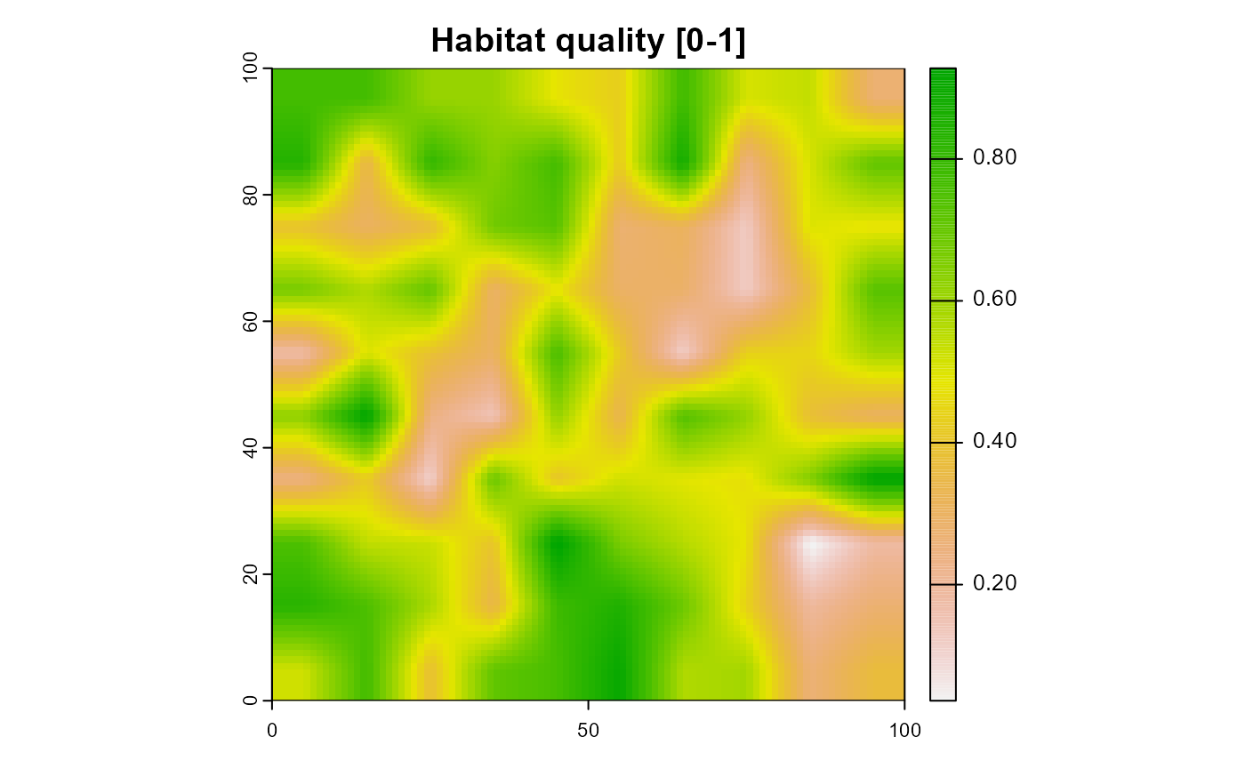

Figure 5: The habitat quality of the example landscape. Only the first layer of 10 identical ones is shown.

Pre-setup

Before creating the simulation, it may be helpful to enable extensive reporting, which will print out a lot of information each time a metaRange function is called. This can be enabled or disabled at any time (i.e. also while the simulation is running), but in order to highlight what each function call in this tutorial does, we enable it at the beginnig of the setup.

# 0 = no reporting
# 1 = a bit of info
# 2 = very verbose
set_verbosity(2)

Creating the simulation

After the landscape is loaded, the simulation can be created using the create_simulation() function. The only required argument is source_environment which is the landscape / environment SDS that was created in the first step. One can optionally specify an ID for the simulation and a seed for the random number generator.

sim <- create_simulation(
    source_environment = landscape,
    ID = "example_simulation",
    seed = 1)
#> number of time steps: 10
#> time step layer mapping: 1, 2, 3, 4, 5, 6, 7, 8, 9, 10
#> added environment
#> class       : SpatRasterDataset 
#> subdatasets : 3 
#> dimensions  : 100, 100 (nrow, ncol)
#> nlyr        : 10, 10, 10 
#> resolution  : 1, 1  (x, y)
#> extent      : 0, 100, 0, 100  (xmin, xmax, ymin, ymax)
#> coord. ref. :  
#> source(s)   : memory 
#> names       : temperature, precipitation, habitat
#> 
#> created simulation: example_simulation

If you want to inspect the simulation object, you can either print it, to lists its fields and methods or use the summary() function to get an overview of the simulation state.

sim
#> metaRangeSimulation object
#> Fields: 
#>   $ID
#>   $globals
#>   $environment
#>   $number_time_steps
#>   $time_step_layer
#>   $current_time_step
#>   $queue
#>   $processes
#>   $seed
#> Species: none
#> Methods: 
#>   $species_names()
#>   $add_globals()
#>   $add_species()
#>   $add_traits()
#>   $add_process()
#>   $begin()
#>   $exit()
#>   $set_current_time_step()
#>   $set_time_layer_mapping()
#>   $print()
#>   $summary()
summary(sim)
#> ID: example_simulation 
#> Environment: 
#> class       : SpatRasterDataset 
#> subdatasets : 3 
#> dimensions  : 100, 100 (nrow, ncol)
#> nlyr        : 10, 10, 10 
#> resolution  : 1, 1  (x, y)
#> extent      : 0, 100, 0, 100  (xmin, xmax, ymin, ymax)
#> coord. ref. :  
#> source(s)   : memory 
#> names       : temperature, precipitation, habitat 
#> Time step layer mapping:  1 2 3 4 5 6 7 8 9 10 
#> Current time step:  1 
#> Seed:  1 
#> Species:
#>   
#> Simulation level processes:
#> NULL
#> Gobal variables:
#> NULL
#> Queue:
#> At process:  0 out of:  0 
#> Remaining queue: 
#> --- empty 
#> Future (next time step) queue: 
#> --- empty

Adding species to the simulation

After the simulation is created, species can be added to it using the add_species() function. At this point one has to switch to the earlier mentioned R6 syntax. This means that add_species() is a method of the simulation object and can be called using the $ operator (i.e. by indexing the simulation object and calling a function that is stored inside of it). The only required argument is name which is the name of the species that will be added.

sim$add_species(name = "species_1")
#> adding species
#> Name: species_1

This species can now be accessed by using the $ operator again.

sim$species_1
#> Species:  species_1 
#> processes: 
#> NULL
#> traits: 
#> character(0)

If you want to add more species, you can just repeat the add_species() call.

sim$add_species(name = "species_2")
#> adding species
#> Name: species_2

If you are at any point wondering which, or how many species are in the simulation, you can use the species_names() method.

sim$species_names()
#> [1] "species_2" "species_1"

Adding traits to species

After species are added to the simulation, traits can be asigned to them using the add_traits() method. This function is able to add (multiple) traits to multiple species at once, which is useful when setting up a large number of species with the same traits. The first argument is species which is a character vector of the species names to which the trait should be assigned to. The second argument is population_level, which decides on what “level” the trait should be added. If TRUE, the trait will be expanded to fill the whole landscape (i.e. one value per population). All following arguments can be supplied in the form of trait_name = trait_value.

sim$add_traits(
    species = c("species_1", "species_2"),
    population_level = TRUE,
    abundance = 500,
    climate_suitability = 1,
    reproduction_rate = 0.3,
    carrying_capacity = 1000
    # ...
    # Note that here could be more traits, there is no limit
)
#> adding traits:
#> [1] "abundance"           "climate_suitability" "reproduction_rate"  
#> [4] "carrying_capacity"
#> 
#> to species:
#> [1] "species_1" "species_2"
#>

Some traits may not require to be stored at the population level, e.g. if they are a property of the species as a whole. In this case, population_level can be set to FALSE and the trait will be added as-is, without further processing. For this example we assume that both species have the same dispersal kernel that it is constant over the whole landscape (i.e. the same for each population). In case one is unfamiliar with the concept of dispersal kernels, a good introduction is “Nathan, R., Klein, E., Robledo-Arnuncio, J.J. & Revilla, E. (2012) Dispersal kernels: review” [Ref. 1], but on a basic level, a dispersal kernel is a matrix that describes the dispersal probability from a source population to its surrounding habitat. We can use the function calculate_dispersal_kernel() to create such a dispersal kernel and then add it to both species. Note that we can call calculate_dispersal_kernel() directly in the add_traits() call.

sim$add_traits(
    species = c("species_1", "species_2"),
    population_level = FALSE,
    dispersal_kernel = calculate_dispersal_kernel(
        # in grid cells
        max_dispersal_dist = 3,
        # the function to use to calculate the kernel values
        kfun = negative_exponential_function,
        # in grid cells
        mean_dispersal_dist = 1
    )
)
#> adding traits:
#> [1] "dispersal_kernel"
#> 
#> to species:
#> [1] "species_1" "species_2"
#>

Assuming we are interested to find out how the two species would inhabit our landscape, we can give both of them different environmental preferences for the two envionmental variables in the simulation environment (temperature & precipitation). Note that the names of the traits are arbitrary and can be chosen by the user and that there is no predetermined connection between e.g. “min_temperature” and the temperature variable in the environment. It is the responsibility of the species processes (therfore of the user) to access the correct traits and use them in the correct way, which is why meaningfull trait names are important.

sim$add_traits(
    species = "species_1",
    population_level = FALSE,
    max_temperature = 300, # Kelvin
    optimal_temperature = 288,
    min_temperature = 280,
    max_precipitation = 1000, # mm
    optimal_precipitation = 700,
    min_precipitation = 200
)
#> adding traits:
#> [1] "max_temperature"       "optimal_temperature"   "min_temperature"      
#> [4] "max_precipitation"     "optimal_precipitation" "min_precipitation"
#> 
#> to species:
#> [1] "species_1"
#> 
sim$add_traits(
    species = "species_2",
    population_level = FALSE,
    max_temperature = 290,
    optimal_temperature = 285,
    min_temperature = 270,
    max_precipitation = 1000,
    optimal_precipitation = 500,
    min_precipitation = 0
)
#> adding traits:
#> [1] "max_temperature"       "optimal_temperature"   "min_temperature"      
#> [4] "max_precipitation"     "optimal_precipitation" "min_precipitation"
#> to species:
#> [1] "species_2"
#>

Adding processes

After the species and their traits are added, the processes that describe the species interaction with their environment can be added, using the add_processes() method. The arguments are: species which is a character vector of the species that should get the process, process_name which is a human readable name for the process and process_fun which is the function that will be executed when the process is called. One argument that might be confusing is the execution_priority. This is a number that gives the process a priority “weight” and decides in which order the processes are executed within one time step. The smaller the number, the earlier the process will be executed (e.g. 1 gets executed before 2). In the case two processes have the same priority, it is assumed that they are independent from each other and that their execution order doesn’t matter. They will be executed in alphabetical order. (Technical note: Don’t count on this behavior, it may change in the future. Equal priority means it should not matter in what order they are executed).

In this example we will first add three basic processes to each species, one for estimating the suitability of a habitat cell, one that calculates the population growth and one that describes the dispersal. To calculate the suitability, we use the metaRange function calculate_suitability() that was adapted from a formula published by Yin et al. in 1995 [Ref. 2] and simplified by Yan and Hunt in 1999 (eq:4) [Ref. 3]. The formula takes the three cardinal values of environmental niche (minimum tolerable value, optimal vale and maximum tolerable value) and constructs a suitability curve based on a beta distribution. In the following code we do this for both the precipitation and the temperature and then multiply the values to get a joint suitability over the two environmental niches. The user could also define their own function to calculate the suitability.

Note the use of the self keyword in the function. In this context, self refers to the species that the process is attached to. This means that the function can access the species traits and modify them and also access the environment (each species holds a reference to the simulation it was created in).

Suitability

sim$add_process(
    species = c("species_1", "species_2"),
    process_name = "calculate_suitability",
    process_fun = function() {
        self$traits$climate_suitability <-
            calculate_suitability(
                self$traits$max_temperature,
                self$traits$optimal_temperature,
                self$traits$min_temperature,
                # The following acceses the "current" environment
                # of a time step
                # (i.e. from the raster layer, that corresponds
                # to the current time step)
                # For user convenice, this "current" environment
                # is converted to a plain matrix,
                # to allow easier calculations
                self$sim$environment$current$temperature
            ) *
            calculate_suitability(
                self$traits$max_precipitation,
                self$traits$optimal_precipitation,
                self$traits$min_precipitation,
                self$sim$environment$current$precipitation
            )
    },
    execution_priority = 1
)
#> adding process: calculate_suitability
#> to species:
#> [1] "species_1" "species_2"
#>

Reproduction

For the reproduction process we can use a built in function ricker_reproduction_model() that implements the “classic” Ricker reproduction model (Ricker, W.E. (1954) compare also: Cabral, J.S. and Schurr, F.M. (2010)) [Ref. 4 & 5].

sim$add_process(
    species = c("species_1", "species_2"),
    process_name = "reproduction",
    process_fun = function() {
        # first let the carrying capacity
        # depend on the climate suitability
        self$traits$carrying_capacity <-
            self$traits$carrying_capacity *
            self$traits$climate_suitability

        # let the reproduction rate
        # depend on the habitat quality
        self$traits$reproduction_rate <-
            self$traits$reproduction_rate *
            self$sim$environment$current$habitat

        # use a ricker reproduction model
        # to calculate the new abundance
        self$traits$abundance <-
            ricker_reproduction_model(
                self$traits$abundance,
                self$traits$reproduction_rate,
                self$traits$carrying_capacity
            )
    },
    execution_priority = 2
)
#> adding process: reproduction
#> to species:
#> [1] "species_1" "species_2"
#>

Dispersal

To apply the dispersal kernel to the abundance of the species, we can use the dispersal() function. It takes the dispersal kernel and applies it to each population (grid cell) of the species and then returns the dispersed abundance. In other fields this process is known as a 2D convolution and e.g. used when blurring an image. Therfore one can think of the dispersal in a similar way, as a “blurring” of the species abundance over the landscape. Note that you can also use [[ indexing to access the traits of a species (which is actually slightly faster than $ indexing).

sim$add_process(
    species = c("species_1", "species_2"),
    process_name = "dispersal_process",
    process_fun = function() {
        self$traits[["abundance"]] <- dispersal(
            abundance = self$traits[["abundance"]],
            dispersal_kernel = self$traits[["dispersal_kernel"]])
    },
    execution_priority = 3
)
#> adding process: dispersal_process
#> to species:
#> [1] "species_1" "species_2"
#>

Executing the simulation

After all species, traits and processes are added to the simulation, it can be executed via the begin() method. To reduce the amount of output while the simulation is running, we’ll set the verbosity to 1.

set_verbosity(1)
sim$begin()
#> Starting simualtion.
#> start of time step: 1
#> end of time step: 1
#> 0.41 secs remaining (estimate)
#> 10 % done
#> start of time step: 2
#> end of time step: 2
#> 0.58 secs remaining (estimate)
#> 20 % done
#> start of time step: 3
#> end of time step: 3
#> 0.34 secs remaining (estimate)
#> 30 % done
#> start of time step: 4
#> end of time step: 4
#> 0.28 secs remaining (estimate)
#> 40 % done
#> start of time step: 5
#> end of time step: 5
#> 0.22 secs remaining (estimate)
#> 50 % done
#> start of time step: 6
#> end of time step: 6
#> 0.22 secs remaining (estimate)
#> 60 % done
#> start of time step: 7
#> end of time step: 7
#> 0.16 secs remaining (estimate)
#> 70 % done
#> start of time step: 8
#> end of time step: 8
#> 0.1 secs remaining (estimate)
#> 80 % done
#> start of time step: 9
#> end of time step: 9
#> 0.043 secs remaining (estimate)
#> 90 % done
#> start of time step: 10
#> end of time step: 10
#> 0 secs remaining (estimate)
#> 100 % done
#> Simulation: 'example_simulation' finished
#> Exiting the Simulation
#> Runtime: 0.52 secs

Plotting the results

To investigate the results, you can use the plot() function. Note that the following two functions essentially plot the same, the only difference is that the first one calls plot() on the simulation object while the second one calls plot() on the species object

# define a nice color palette
plot_cols <- hcl.colors(100, "Purple-Yellow", rev = TRUE)
plot(
    sim,
    obj = "species_1",
    name = "abundance",
    main = "Species 1: abundance",
    col = plot_cols
)

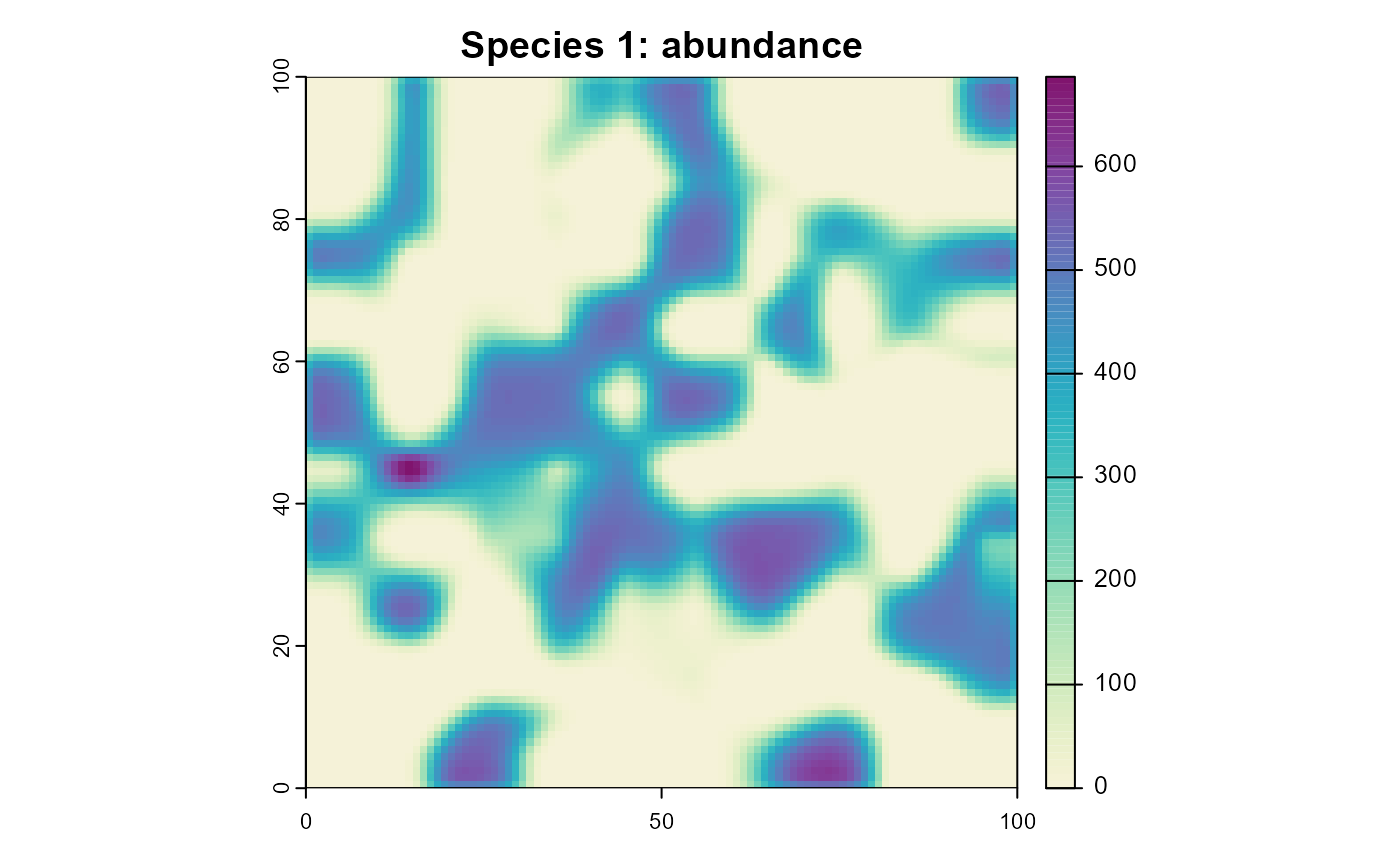
Figure 6: The resulting abundance distribution of species 1 after 10 simulation time steps.

plot(
    sim$species_2,
    trait = "abundance",
    main = "Species 2: abundance",
    col = plot_cols
)

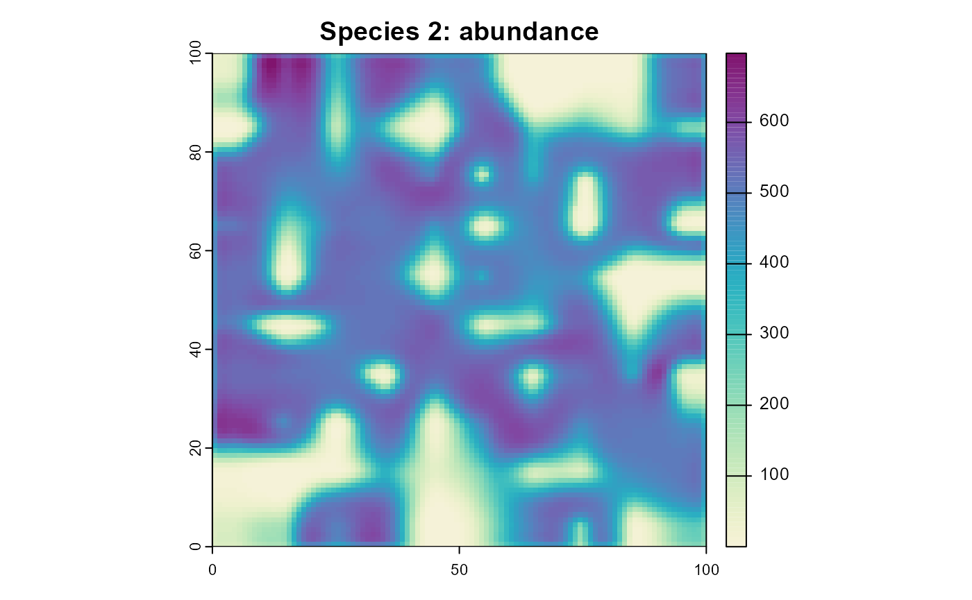
Figure 7: The resulting abundance distribution of species 2 after 10 simulation time steps.

Saving the simulation

To save results you can use the save_species() function. This will save the (possibly specified) traits of a species, either as a raster (.tif) or as a text (.csv) file, whatever is more appropriate for the data. Note that this function does not save the species processes. One should keep a copy of the script that is used to run the simulation to make it repeatable.

save_species(
    sim$species_1,
    traits = c("name", "of", "one_or_more", "traits"),
    path = "path/to/a/folder/"
)

References

Nathan, R., Klein, E., Robledo-Arnuncio, J.J. and Revilla, E. (2012) Dispersal kernels: review. in: Dispersal Ecology and Evolution pp. 187–210. (eds J. Clobert, M. Baguette, T.G. Benton and J.M. Bullock), Oxford, UK: Oxford Academic, 2013. doi:10.1093/acprof:oso/9780199608898.003.0015
Yin, X., Kropff, M.J., McLaren, G., Visperas, R.M., (1995) A nonlinear model for crop development as a function of temperature, Agricultural and Forest Meteorology, Volume 77, Issues 1-2, Pages 1–16, doi:10.1016/0168-1923(95)02236-Q
Yan, W., Hunt, L.A. (1999) An Equation for Modelling the Temperature Response of Plants using only the Cardinal Temperatures, Annals of Botany, Volume 84, Issue 5, Pages 607–614, ISSN 0305-7364, doi:10.1006/anbo.1999.0955
Ricker, W.E. (1954) Stock and recruitment. Journal of the Fisheries Research Board of Canada, 11, 559–623. doi:10.1139/f54-039
Cabral, J.S. and Schurr, F.M. (2010) Estimating demographic models for the range dynamics of plant species. Global Ecology and Biogeography, 19, 85–97. doi:10.1111/j.1466-8238.2009.00492.x

Appendix

Here is the function that is used to generate the example landscape.

create_example_landscape <- function() {
    set.seed(3)
    create_land <- function() {
        sample_size <- 100
        n_cells <- 100
        res <- terra::disagg(
            terra::rast(
                matrix(
                    sample.int(
                        sample_size,
                        n_cells,
                        replace = TRUE,
                        prob = sin(seq(0.05, pi-0.05, length.out = sample_size))
                    ),
                    nrow = sqrt(n_cells),
                    ncol = sqrt(n_cells)
                )
            ),
            10,
            "bilinear"
        )  / 100
        ext(res) <- c(0, 100, 0, 100)
        return(res)
    }
    temperature <- create_land() * 20 + 273.15
    temperature <- rep(temperature, 10)
    precipitation <- create_land() * 1000
    precipitation <- rep(precipitation, 10)
    habitat <- create_land()
    habitat <- rep(habitat, 10)
    landscape <- terra::sds(temperature, precipitation, habitat)
    names(landscape) <- c("temperature", "precipitation", "habitat")
    return(landscape)
}

Fallert, S. and Cabral, J.S.