05: Directed (weighted) dispersal

Fallert, S. and Cabral, J.S.

While the assumption of dispersal via a static kernel is an often used simplification, it is not always appropriate. For many species, dispersal is not solely random, but directed towards a specific target or influenced by other external factors. To allow simulations that include this, the dispersal() function gives the user the option to supply a third argument, weights, which is used to redistribute the individuals within the dispersal kernel. If supplied, the weights needs to be a matrix of the same dimensions as environment and the values should be in the range of [0-1]. One could for example use calculate_suitability() to create a matrix that represent a general habitat suitability and use it as weights, which would correspond to an ecological meaning of “individuals moving towards a more suitable habitat during dispersal, if they have the ability to reach it”.

Basic setup

library(metaRange)
#> metaRange version: 0.0.0.9000
library(terra)
#> terra 1.7.55

Setup the basic simulation with two identical species.

sim <- create_simulation(create_example_landscape())
sim$add_species("species_1")
sim$add_species("species_2")
sim$add_traits(
    species = c("species_1", "species_2"),
    abundance = 100,
    climate_suitability = 1
)
sim$add_traits(
    species = c("species_1", "species_2"),
    population_level = FALSE,
    max_temperature = 300,
    optimal_temperature = 288,
    min_temperature = 280,
    max_precipitation = 1000,
    optimal_precipitation = 700,
    min_precipitation = 200,
    dispersal_kernel = calculate_dispersal_kernel(
        max_dispersal_dist = 12,
        kfun = negative_exponential_function,
        mean_dispersal_dist = 6
    )
)
sim$add_process(
    species = c("species_1", "species_2"),
    process_name = "calculate_suitability",
    process_fun = function() {
        self$traits$climate_suitability <-
            calculate_suitability(
                self$traits$max_temperature,
                self$traits$optimal_temperature,
                self$traits$min_temperature,
                self$sim$environment$current$temperature
            ) *
            calculate_suitability(
                self$traits$max_precipitation,
                self$traits$optimal_precipitation,
                self$traits$min_precipitation,
                self$sim$environment$current$precipitation
            )
    },
    execution_priority = 1
)
sim$add_process(
    species = c("species_1", "species_2"),
    process_name = "reproduction",
    process_fun = function() {
        self$traits[["abundance"]] <-
            self$traits[["abundance"]] *
            self$traits[["climate_suitability"]]
    },
    execution_priority = 2
)

Now we add the two methods of dispersal to the two species to highlight the difference.

Unweighted dispersal

sim$add_process(
    species = "species_1",
    process_name = "dispersal_process",
    process_fun = function() {
        self$traits[["abundance"]] <- dispersal(
            abundance = self$traits[["abundance"]],
            dispersal_kernel = self$traits[["dispersal_kernel"]]
        )
    },
    execution_priority = 3
)

Weighted dispersal

sim$add_process(
    species = "species_2",
    process_name = "dispersal_process",
    process_fun = function() {
        self$traits[["abundance"]] <- dispersal(
            abundance = self$traits[["abundance"]],
            dispersal_kernel = self$traits[["dispersal_kernel"]],
            weights = self$traits[["climate_suitability"]]
        )
    },
    execution_priority = 3
)

Comparison of the results

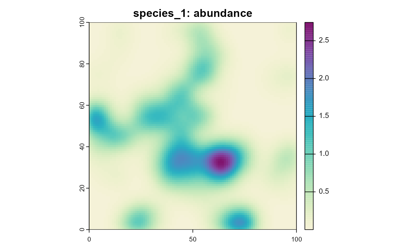
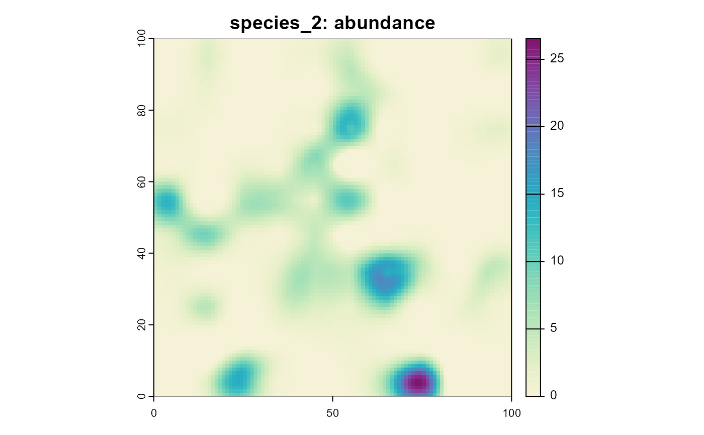
To see the effect, we run the simulation for 10 time steps and plot the results.

sim$begin()
plot_cols <- hcl.colors(100, "Purple-Yellow", rev = TRUE)
plot(sim, "species_1", "abundance", col = plot_cols)
plot(sim, "species_2", "abundance", col = plot_cols)

Note how the plot for species two is less “blurry” and the different scales of the two plots. While the first species looses individuals by dispersing in unsuitable habitat, the second species can keep a much larger population size, by moving towards more suitable habitat during dispersal.