04: Metabolic scaling

The temperature of the environment where a species lives (and their bodymass) can have a large impact on their metabolism and in consequence also on different processes such as growth, reproduction and mortality. To include this effect, metaRange offers the option to use metabolic scaling based on the “metabolic theory of ecology” described by Brown et al. (2004) [Ref: 1] in the following form: \[{parameter = normalization\_constant \cdot mass^{scaling\_exponent} \cdot e^{\frac{E}{k \cdot temperature}}}\] This is implemented in the function metabolic_scaling(), which can be used to calculate the parameter value for any metabolically influenced process, based on the mean individual body mass of a population, a process specific constant and the temperature of the environment. It has to be noted that different processes have different activation energy values and scaling exponents.

Parameter	Scaling exponent	Activation energy
resource usage	3/4	-0.65
reproduction, mortality	-1/4	-0.65
carrying capacity	-3/4	0.65

Table 1: Common parameter and their associated scaling exponents and activation energies. Source: table 4 in Brown, J.H., Sibly, R.M. and Kodric-Brown, A. (2012) [Ref: 2]

Calculating the normalization constant

In the absence of experimentally measured values for the normalization constant, metaRange offers the function calculate_normalization_constant() to calculate the normalization constant based on an estimated value for the parameter under a reference temperature.

Example

library(metaRange)
#> metaRange version: 0.0.0.9000
library(terra)
#> terra 1.7.55

Setup the basic simulation.

sim <- create_simulation(create_example_landscape())
sim$add_species("sp1")

Define some basic traits.

sim$add_traits(
    species = "sp1",
    population_level = FALSE,
    "suitability" = NA_real_,
    "temperature_maximum" = 30 + 273,
    "temperature_optimum" = 20 + 273,
    "temperature_minimum" = 0 + 273,
    "precipitation_maximum" = 1200,
    "precipitation_optimum" = 800,
    "precipitation_minimum" = 0
)

Add the parameter used in the metabolic scaling as global variables, since they are not species specific.

sim$add_globals(
    "E_reproduction_rate" = -0.65,
    "E_carrying_capacity" = 0.65,
    "exponent_reproduction_rate" = -1 / 4,
    "exponent_carrying_capacity" = -3 / 4,
    "k" = 8.617333e-05
)

Add traits that are used in the reproduction model including an estimate of the reproduction rate and the carrying capacity.

sim$add_traits(
    species = "sp1",
    population_level = TRUE,
    "abundance" = 100,
    "reproduction_rate" = 0.5,
    "carrying_capacity" = 1000,
    "mass" = 1
)

Calculate the normalization constant, based on the parameter estimate and the optimal temperature of the species. Note that this could also be done in a loop over multiple species.

sim$add_traits(
    species = "sp1",
    population_level = FALSE,
    "reproduction_rate_mte_constant" = calculate_normalization_constant(
        parameter_value =
            sim$sp1$traits[["reproduction_rate"]][[1]],
        scaling_exponent =
            sim$globals[["exponent_reproduction_rate"]],
        mass =
            sim$sp1$traits[["mass"]][[1]],
        reference_temperature =
            sim$sp1$traits[["temperature_optimum"]],
        E =
            sim$globals[["E_reproduction_rate"]],
        k =
            sim$globals[["k"]]
    ),
    "carrying_capacity_mte_constant" = calculate_normalization_constant(
        parameter_value =
            sim$sp1$traits[["carrying_capacity"]][[1]],
        scaling_exponent =
            sim$globals[["exponent_carrying_capacity"]],
        mass =
            sim$sp1$traits[["mass"]][[1]],
        reference_temperature =
            sim$sp1$traits[["temperature_optimum"]],
        E =
            sim$globals[["E_carrying_capacity"]],
        k =
            sim$globals[["k"]]
    )
)

Add a process that does the metabolic scaling in each time step.

sim$add_process(
    species = "sp1",
    process_name = "mte",
    process_fun = function() {
        self$traits[["reproduction_rate"]] <- metabolic_scaling(
            normalization_constant =
                self$traits[["reproduction_rate_mte_constant"]],
            scaling_exponent =
                self$sim$globals[["exponent_reproduction_rate"]],
            mass =
                self$traits[["mass"]],
            temperature =
                self$sim$environment$current[["temperature"]],
            E =
                self$sim$globals[["E_reproduction_rate"]],
            k =
                self$sim$globals[["k"]]
        )

        self$traits[["carrying_capacity"]] <- metabolic_scaling(
            normalization_constant =
                self$traits[["carrying_capacity_mte_constant"]],
            scaling_exponent =
                self$sim$globals[["exponent_carrying_capacity"]],
            mass =
                self$traits[["mass"]],
            temperature =
                self$sim$environment$current[["temperature"]],
            E =
                self$sim$globals[["E_carrying_capacity"]],
            k =
                self$sim$globals[["k"]]
        )
    },
    execution_priority = 2
)

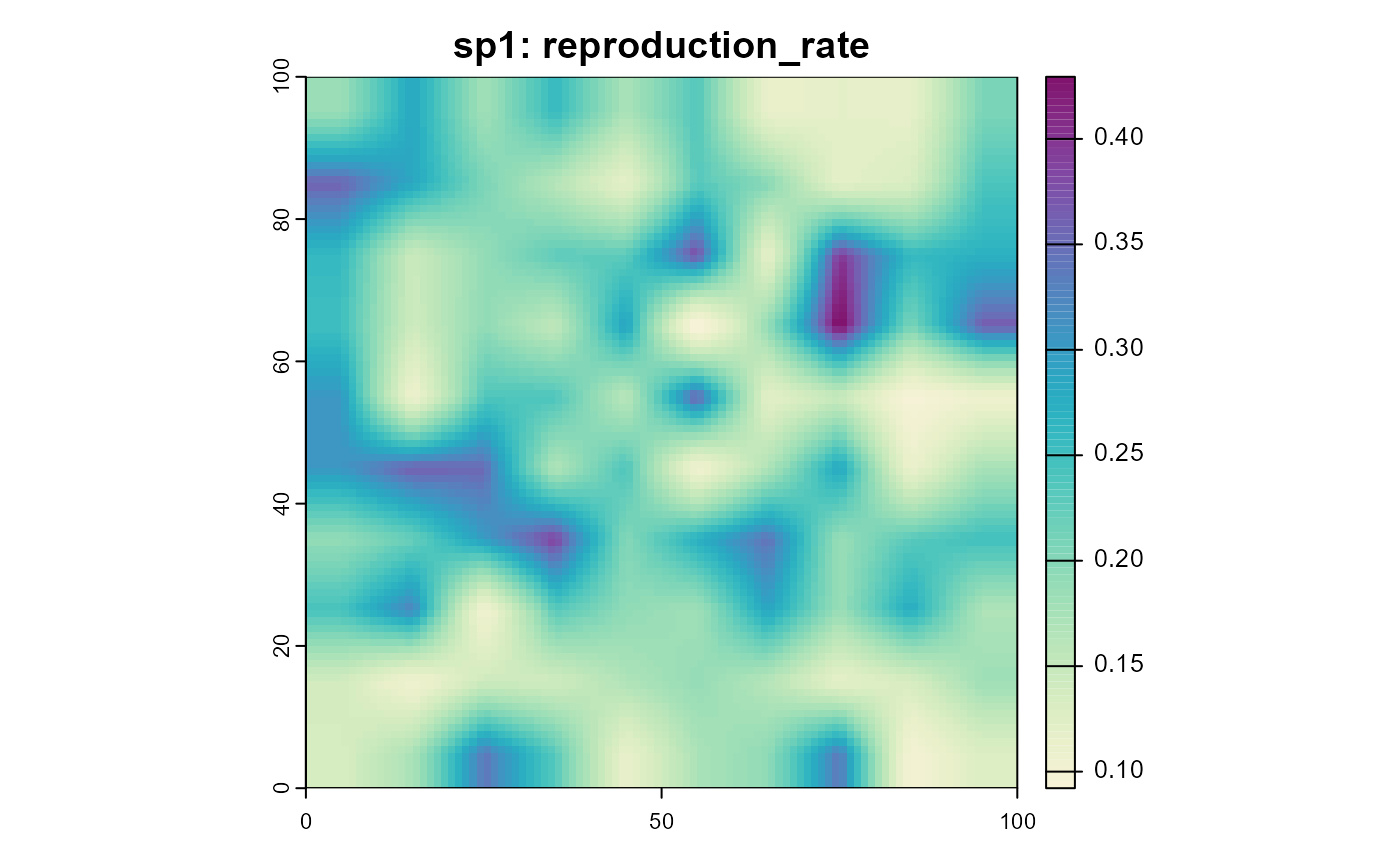
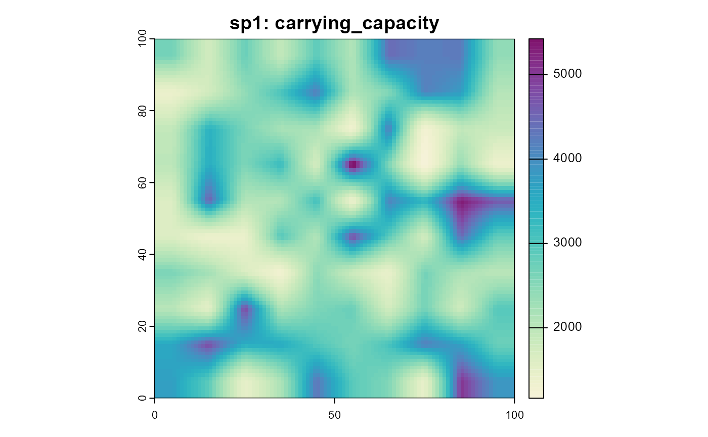
After this point, processes could be added that use the scaled parameters. Here we just plot the scaled parameter instead.

sim$set_time_layer_mapping(c(1, 2))
sim$begin()
plot_cols <- hcl.colors(100, "Purple-Yellow", rev = TRUE)
plot(sim, "sp1", "reproduction_rate", col = plot_cols)
plot(sim, "sp1", "carrying_capacity", col = plot_cols)

Note that these results show an “everything else equal” scenario, where the only variable is the temperature. In a more realistic scenario, the suitability of the habitat might also influence the reproduction rate and carrying capacity or the mean individual body mass might change with the temperature and change the results.

References

Brown, J.H., Gillooly, J.F., Allen, A.P., Savage, V.M. and West, G.B. (2004), Toward a Metabolic Theory of Ecology. Ecology, 85: 1771-1789. https://doi.org/10.1890/03-9000
Brown, J.H., Sibly, R.M. and Kodric-Brown, A. (2012). Introduction: Metabolism as the Basis for a Theoretical Unification of Ecology. In: Metabolic Ecology (eds R.M. Sibly, J.H. Brown and A. Kodric-Brown). https://doi.org/10.1002/9781119968535.ch

Fallert, S. and Cabral, J.S.

Calculating the normalization constant

Example

References