07: Age structured populations
Fallert, S. and Cabral, J.S.
Source:vignettes/A07_age_structured_populations.Rmd
A07_age_structured_populations.RmdMany species have population dynamics that require more complex equations than the simple Ricker model (which describes overcompensatory scramble competition with non-overlapping generations). A common abstraction to deal with this complexity is to partition a species into functional subgroups that undergo different processes. This could for example be juveniles who are dispersing and looking for a habitat, who then become adults who are stationary but have the ability to reproduce and generate the next generation of juveniles. The following illustrates a simple example on how one could model such a system with metaRange.
Basic setup
Setup the basic simulation.
raster_file <- system.file("ex/elev.tif", package = "terra")
r <- rast(raster_file)
habitat <- scale(r, center = FALSE, scale = TRUE)
habitat <- rep(habitat, 10)
landscape <- sds(habitat)
names(landscape) <- "habitat"
sim <- create_simulation(landscape)
sim$add_species("species_1")
Traits
Now we add the traits for both the juveniles and the adults.
sim$add_traits(
    species = "species_1",
    n_juveniles = 100,
    n_adults = 100,
    mortality_juveniles = 0.1,
    mortality_adults = 0.7,
    reproduction_rate = 2
)
sim$add_traits(
    species = "species_1",
    population_level = FALSE,
    dispersal_kernel = calculate_dispersal_kernel(
        max_dispersal_dist = 8,
        kfun = negative_exponential_function,
        mean_dispersal_dist = 4
    )
)
Processes
The important part of this age structured population model is the transition between the age classes. These processes could of course be of any desired complexity, but to make the example easier to follow, here we will just use simple functions:
sim$add_process(
    species = "species_1",
    process_name = "reproduction",
    process_fun = function() {
        self$traits[["n_juveniles"]] <-
            self$traits[["n_adults"]] + (
                self$traits[["n_adults"]] * self$traits[["reproduction_rate"]]
            ) * self$sim$environment$current$habitat
    },
    execution_priority = 1
)
sim$add_process(
    species = "species_1",
    process_name = "maturation",
    process_fun = function() {
        self$traits[["n_adults"]] <-
            self$traits[["n_adults"]] +
            self$traits[["n_juveniles"]] * (1 - self$traits[["mortality_juveniles"]])
    },
    execution_priority = 3
)
More processes
As mentioned in the introduction paragraph, we will add a dispersal
process for the juveniles and an aditional process controlling the
mortality of the adults. Note that we do not need to add an
mortality_of_juveniles process, since their mortality is
already included in the maturation process.
sim$add_process(
    species = "species_1",
    process_name = "dispersal_of_juveniles",
    process_fun = function() {
        self$traits[["n_juveniles"]] <- dispersal(
            abundance = self$traits[["n_juveniles"]],
            dispersal_kernel = self$traits[["dispersal_kernel"]]
        )
    },
    execution_priority = 2
)
sim$add_process(
    species = "species_1",
    process_name = "mortality_of_adults",
    process_fun = function() {
        self$traits[["n_adults"]] <-
            self$traits[["n_adults"]] * (1 - self$traits[["mortality_adults"]])
    },
    execution_priority = 4
)
Result
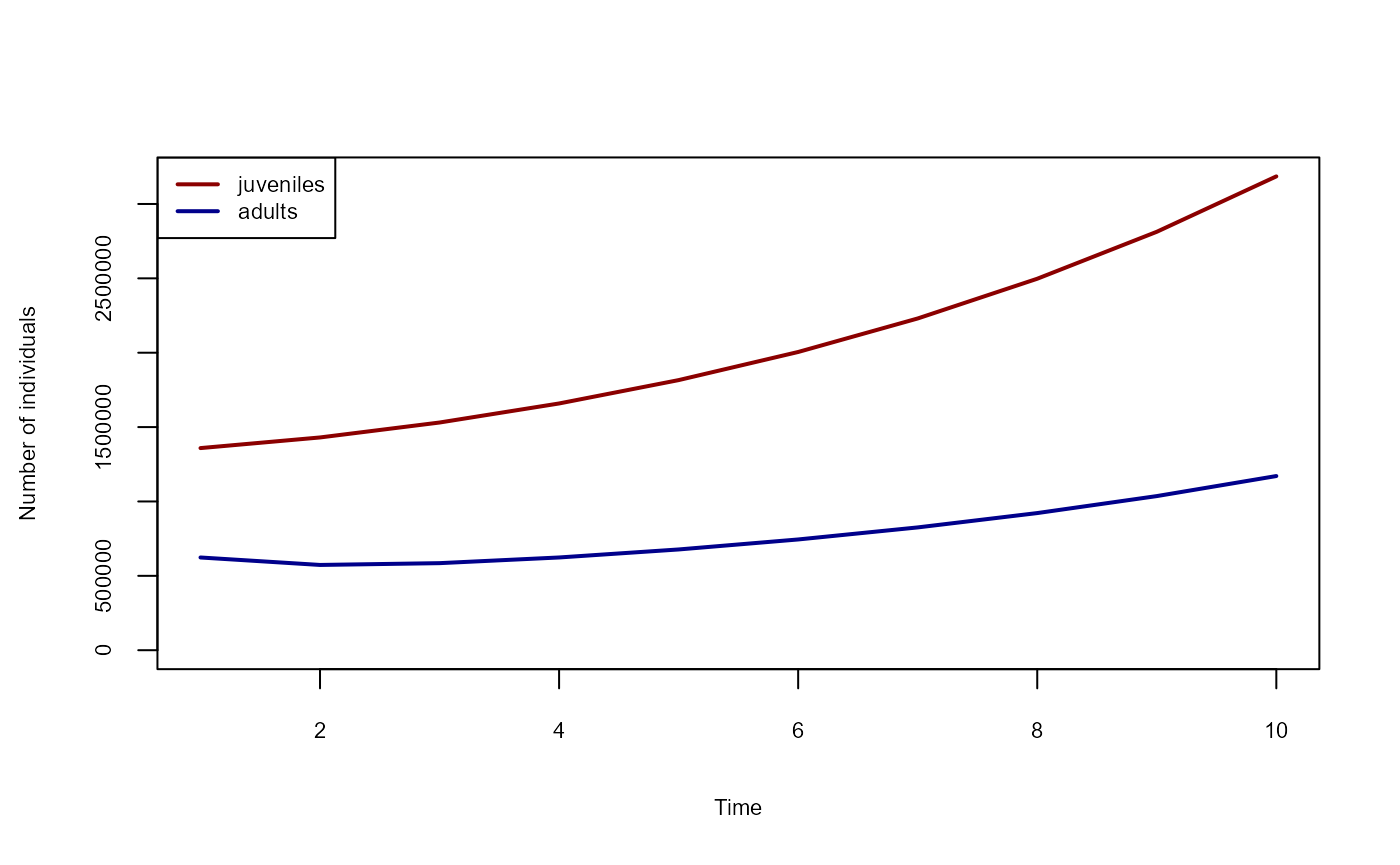
Lastly, we add a process that reports the numbers of adults and juveniles over time, after which we can execute the simulation and plot the results.
sim$add_globals(n_juveniles = c(), n_adults = c())
sim$add_process(
    process_name = "logger",
    process_fun = function() {
        self$globals$n_juveniles <-
            c(self$globals$n_juveniles, sum(self$species_1$traits[["n_juveniles"]]))
        self$globals$n_adults <-
            c(self$globals$n_adults, sum(self$species_1$traits[["n_adults"]]))
    },
    execution_priority = 5
)
sim$begin()
plot(
    1:10,
    sim$globals$n_juveniles,
    col = "darkred",
    type = "l",
    lwd = 2,
    ylim = c(0, max(sim$globals$n_juveniles, sim$globals$n_adults)),
    xlab = "Time",
    ylab = "Number of individuals",
    cex.lab = 0.7,
    cex.axis = 0.7
)
lines(1:10, sim$globals$n_adults, col = "darkblue", lwd = 2)
legend(
    "topleft",
    legend = c("juveniles", "adults"),
    col = c("darkred", "darkblue"),
    lty = 1,
    lwd = 2,
    cex = 0.7
)