Dispersal is a key process in the life cycle of many species and can
have a large impact on the (meta) population dynamics and the ability of
a species to survive in and adapt to a changing environment.
metaRange allows the user to simulate dispersal in two
different ways using the dispersal() function, which are
described in the following sections.
Since metaRange is not an individual based model it uses the concept of a dispersal kernel to simulate dispersal for each population. If one is not familiar with this topic, a good introduction is “Nathan, Klein, Robledo-Arnuncio, & Revilla (2012) Dispersal kernels: review” [Ref. 1].
To also give a short explanation here: A dispersal kernel is basically a matrix that describes how likely it is for an individual of a source population (the cell in the center of the matrix) to move to its surrounding habitat (the cells towards the sides of the matrix). To calculate the dispersal of in the whole landscape, this kernel is iteratively centered on each cell of the abundence matrix (i.e. the central cell in the kernel is overlapping with the cell for which we want to calculate the dispersal), and then the abundance of this cell is multiplied with the values in the kernel. Since the kernel is a probability distribution, the result is the number of individuals that move from to central cell outwards (and also the number of individuals that stay in the source cell). This process is repeated for each cell and then all the individual dispersal events are summed up to generate the new abundance matrix after the dispersal. Conceptionally, this process is similar to applying a blur filter to an image in image processing (i.e. “blurring”) or to the mathematical operation of “convolution”.
We can use the function calculate_dispersal_kernel() to
create such a dispersal kernel. This function creates a matrix that has
max_dispersal_dist rows and columns on both sides of the
source cell and expects another function as input that it calls for each
of those cells with the distance from the source cell as an argument.
This may sound complicated but the code is very short if we use the
built-in negative_exponential_function:
max_dispersal_distance <- 10
mean_dispersal_distance <- 7
dispersal_kernel <- metaRange::calculate_dispersal_kernel(
    max_dispersal_dist = max_dispersal_distance, # units: grid cells
    kfun = metaRange::negative_exponential_function, # this function calculates the kernel values
    mean_dispersal_dist = mean_dispersal_distance # this is passed to the kfun
)
We can plot the kernel to get a better understanding of what it looks like. As you can see in the plot, the dispersal kernel is symmetrical around the source cell and the probability of dispersal decreases with the distance from the source cell. The sum of all values in the kernel is 1, which means that the total abundance of the species is conserved during dispersal.
terra::plot(
    terra::rast(
        dispersal_kernel,
        extent = terra::ext(
            -max_dispersal_distance, max_dispersal_distance,
            -max_dispersal_distance, max_dispersal_distance
        )
    ),
    main = "Dispersal probability"
)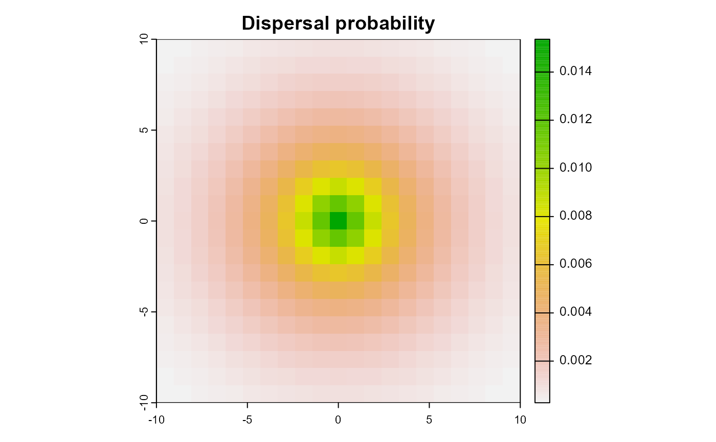
Figure 1: Example dispersal kernel for a negative exponential function
While the assumption of dispersal via such a static kernel is an
often used simplification (i.e. the same kernel is applied to every
population), it is not always appropriate. For many species, dispersal
is not solely random, but directed towards a specific target or
influenced by other external factors. To allow simulations that include
this, the dispersal() function gives the user the option to
supply a third argument, weights, which is used to
redistribute the individuals within the dispersal kernel. If supplied,
the weights need to be a matrix of the same dimensions as the
environment and the values should be in the range of
[0-1].
In this example we use calculate_suitability() to create
a matrix that represent a general habitat suitability and use it as
weights, which would correspond to an ecological meaning of “individuals
moving towards a more suitable habitat during dispersal, if they have
the ability to perceive and reach it”.
Basic setup
First, we load the necessary packages and create an example landscape.
library(metaRange)
#> Warning: package 'metaRange' was built under R version 4.3.3
#> metaRange version: 1.1.4
library(terra)
#> terra 1.7.55
set_verbosity(2)

raster_file <- system.file("ex/elev.tif", package = "terra")
r <- rast(raster_file)
temperature <- scale(r, center = FALSE, scale = TRUE) * 10 + 273.15
temperature <- rep(temperature, 10)
landscape <- sds(temperature)
names(landscape) <- c("temperature")
Then we set up the basic simulation with two identical species.
sim <- create_simulation(landscape)
#> number of time steps: 10
#> time step layer mapping: 1, 2, 3, 4, 5, 6, 7, 8, 9, 10
#> added environment
#> class       : SpatRasterDataset
#> subdatasets : 1
#> dimensions  : 90, 95 (nrow, ncol)
#> nlyr        : 10
#> resolution  : 0.008333333, 0.008333333  (x, y)
#> extent      : 5.741667, 6.533333, 49.44167, 50.19167  (xmin, xmax, ymin, ymax)
#> coord. ref. : lon/lat WGS 84 (EPSG:4326)
#> source(s)   : memory
#> names       : temperature
#>
#> created simulation: simulation_5d40820e
sim$add_species("species_1")
#> adding species
#> name: species_1
sim$add_species("species_2")
#> adding species
#> name: species_2
sim$add_traits(
    species = c("species_1", "species_2"),
    abundance = 100,
    climate_suitability = 1,
    reproduction_rate = 0.3,
    carrying_capacity = 1000
)
#> adding traits:
#> [1] "abundance"           "climate_suitability" "reproduction_rate"
#> [4] "carrying_capacity"
#>
#> to species:
#> [1] "species_1" "species_2"
#>
sim$add_traits(
    species = c("species_1", "species_2"),
    population_level = FALSE,
    max_temperature = 300,
    optimal_temperature = 288,
    min_temperature = 280,
    dispersal_kernel = calculate_dispersal_kernel(
        max_dispersal_dist = 7,
        kfun = negative_exponential_function,
        mean_dispersal_dist = 4
    )
)
#> adding traits:
#> [1] "max_temperature"     "optimal_temperature" "min_temperature"
#> [4] "dispersal_kernel"
#> to species:
#> [1] "species_1" "species_2"
#>
sim$add_process(
    species = c("species_1", "species_2"),
    process_name = "calculate_suitability",
    process_fun = function() {
        self$traits$climate_suitability <-
            calculate_suitability(
                self$traits$max_temperature,
                self$traits$optimal_temperature,
                self$traits$min_temperature,
                self$sim$environment$current$temperature
            )
    },
    execution_priority = 1
)
#> adding process: calculate_suitability
#> to species:
#> [1] "species_1" "species_2"
#>
sim$add_process(
    species = c("species_1", "species_2"),
    process_name = "reproduction",
    process_fun = function() {
        self$traits$abundance <-
            ricker_reproduction_model(
                self$traits$abundance,
                self$traits$reproduction_rate * self$traits$climate_suitability,
                self$traits$carrying_capacity * self$traits$climate_suitability
            )
    },
    execution_priority = 2
)
#> adding process: reproduction
#> to species:
#> [1] "species_1" "species_2"
#>
Now we add the two different methods of dispersal to the two species.
Unweighted dispersal
sim$add_process(
    species = "species_1",
    process_name = "dispersal_process",
    process_fun = function() {
        self$traits[["abundance"]] <- dispersal(
            abundance = self$traits[["abundance"]],
            dispersal_kernel = self$traits[["dispersal_kernel"]]
        )
    },
    execution_priority = 3
)
#> adding process: dispersal_process
#> to species:
#> [1] "species_1"
#>
Weighted dispersal
sim$add_process(
    species = "species_2",
    process_name = "dispersal_process",
    process_fun = function() {
        self$traits[["abundance"]] <- dispersal(
            abundance = self$traits[["abundance"]],
            dispersal_kernel = self$traits[["dispersal_kernel"]],
            weights = self$traits[["climate_suitability"]]
        )
    },
    execution_priority = 3
)
#> adding process: dispersal_process
#> to species:
#> [1] "species_2"
#>
Comparison of the results
We run the simulation and plot the results.
set_verbosity(0)
sim$begin()
plot_cols <- hcl.colors(100, "Purple-Yellow", rev = TRUE)
plot(sim, "species_1", "abundance", col = plot_cols)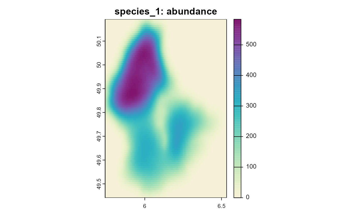
Figure 2: Resulting abundance of species 1 (with unweighted dispersal) after 10 time steps.
plot(sim, "species_2", "abundance", col = plot_cols)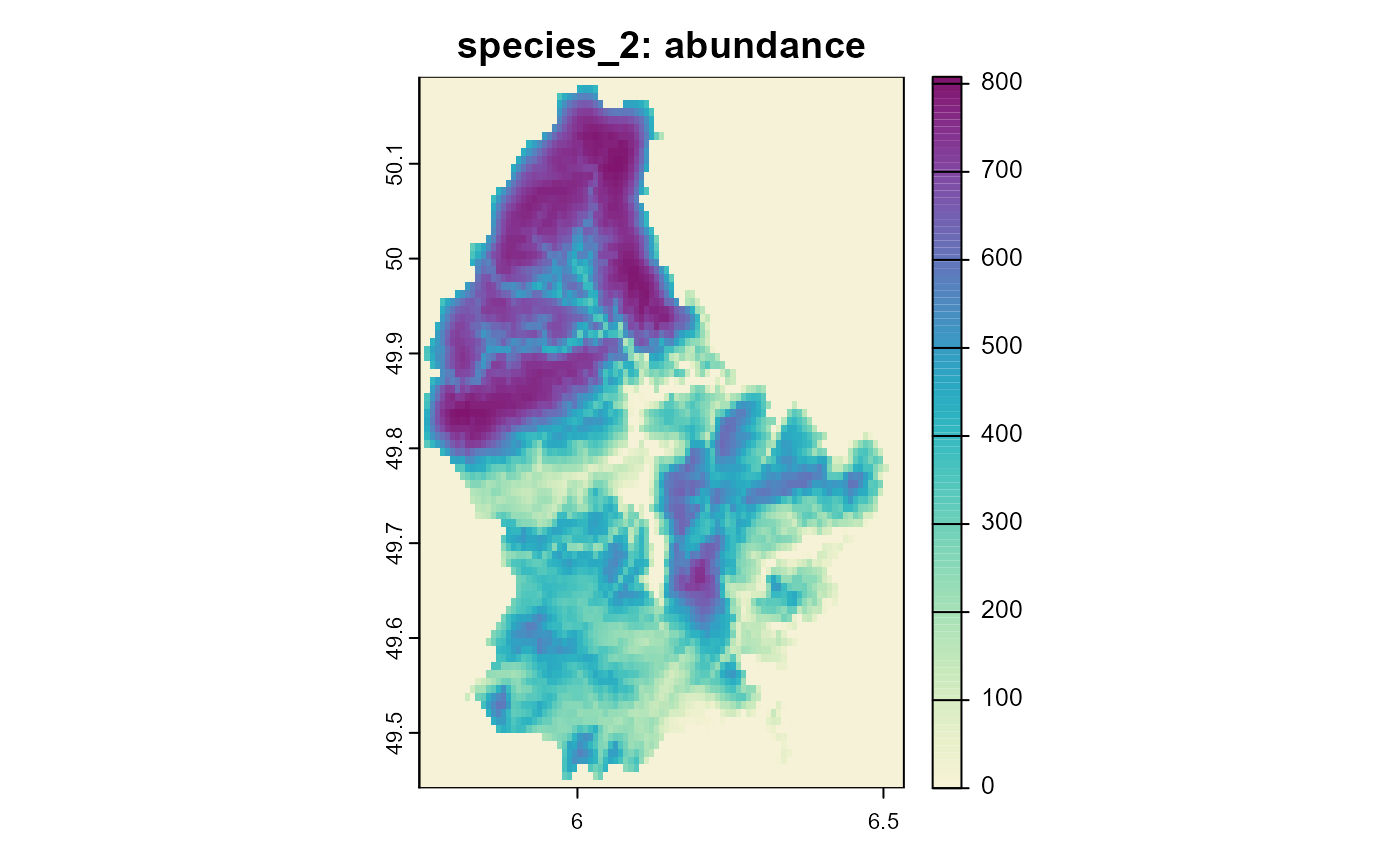
Figure 3: Resulting abundance of species 2 (with weighted dispersal) after 10 time steps.
Note how the plot for species two is less “blurry” and the different scales of the two plots. While the first species loses individuals by dispersing into unsuitable habitat, the second species can keep a much larger population size, by moving towards more suitable habitat during dispersal.
References
- Nathan, R., Klein, E., Robledo-Arnuncio, J.J. and Revilla, E. (2012) Dispersal kernels: review. in: Dispersal Ecology and Evolution pp. 187–210. (eds J. Clobert, M. Baguette, T.G. Benton and J.M. Bullock), Oxford, UK: Oxford Academic, 2013. doi:10.1093/acprof:oso/9780199608898.003.0015