02: Multiple species
Fallert, S. and Cabral, J.S.
Source:vignettes/A02_multiple_species.Rmd
A02_multiple_species.RmdmetaRange is not only able to simulate single species,
but it can also simulate multiple species at the same time. In this
vignette, we will expand our previous example to show how to set up a
multi-species simulation. These species will not interact (that is
explained in a different vignette), but rather be simulated in parallel,
so that we can directly compare how their population development differs
under the same environmental conditions.
Setting up the simulation
As previously, we start by loading the packages and creating the landscape.
library(metaRange)
#> Warning: package 'metaRange' was built under R version 4.3.3
#> metaRange version: 1.1.4
library(terra)
#> terra 1.7.55

# find the file
raster_file <- system.file("ex/elev.tif", package = "terra")

# load it
r <- rast(raster_file)

# scale it
r <- scale(r, center = FALSE, scale = TRUE)

r <- rep(r, 10)
landscape <- sds(r)
names(landscape) <- c("habitat_quality")

# plot the first layer of the landscape
plot(landscape[["habitat_quality"]][[1]], main = "Habitat quality")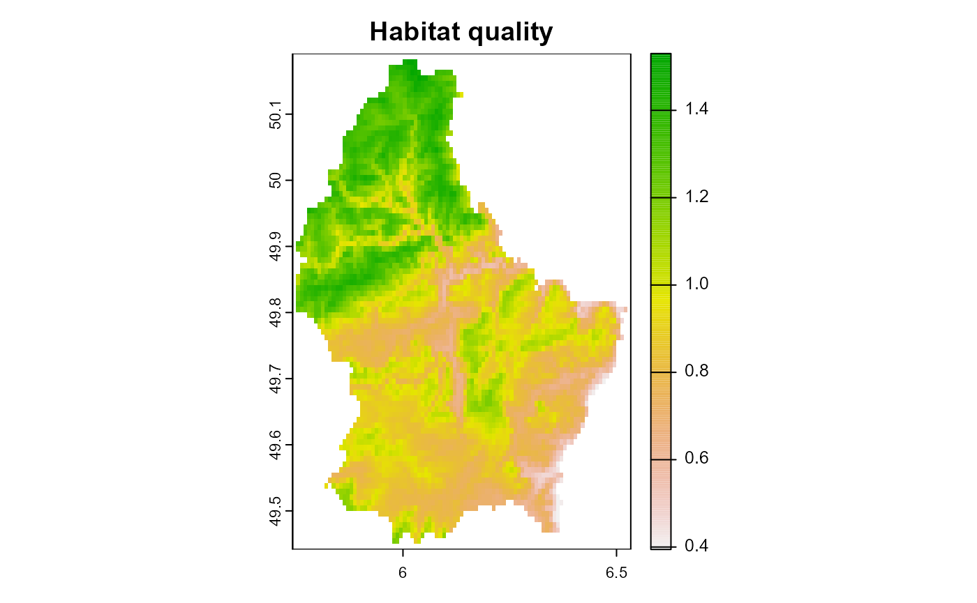
Figure 1: The habitat quality of the example landscape. Note: higher value = better habitat quality
Again, we create a simulation and add the landscape to it.
sim <- create_simulation(
    source_environment = landscape,
    ID = "multiple_species",
    seed = 1
)
Adding more species to the simulation
Instead of only adding one species to the simulation, we can just
supply more names in the add_species() call to create more
species.
sim$add_species(c("species_1", "species_2"))If you are at any point wondering which, or how many species are in
the simulation, you can use the species_names() method.
sim$species_names()
#> [1] "species_2" "species_1"
length(sim$species_names())
#> [1] 2
Adding traits to (multiple) species
The add_traits() method is able to add (multiple) traits
to multiple species at once, which is useful when setting up a large
number of species with the same traits. So instead of only specifying
one species argument, we can specify a vector of species
names, all of which will get the same traits. Here, we set the initial
abundance of the species to be proportional to the habitat quality. This
introduces a new concept of the environemnt: the current
property.
sim$add_traits(
    species = c("species_1", "species_2"),
    population_level = TRUE,
    abundance = 200 * sim$environment$current[["habitat_quality"]]
)
As the name suggests, sim$environment$current[["....."]]
always refers to the “current” state of the landscape (i.e. the
environmental conditions in the present time step). So what is the
difference to the source SDS we used as input to create the
simulation?
- The
sim$environment$sourceSDS[["....."]]is stored as raster data, which has multiple sub-datasets (e.g. habitat quality, temperature, …), multiple layer (one for each time step) and is potentially stored on the disk, which makes it suitable to store large amounts of data (the whole time series), but makes accessing it more complicated and slow. - The
currentenvironment contains a 2 dimensional matrix (i.e. only one / the current layer) for each of the sub-datasets in the source SDS. These matricies are stored and accessible under the same name as the respective data sets in the source SDS and they are stored in memory. This makes it faster and easier to access and them use in calculations (As seen in the code example above).
The current environment is automatically updated at the beginning of each time step, and right now (before the simulation has started) stores the condition of the first time step (i.e. the first layer of each sub-dataset of the sourceSDS).
# define a nice color palette
plot_cols <- hcl.colors(100, "BluYl", rev = TRUE)
plot(
    sim,
    obj = "species_1",
    name = "abundance",
    main = "Initial abundance",
    col = plot_cols
)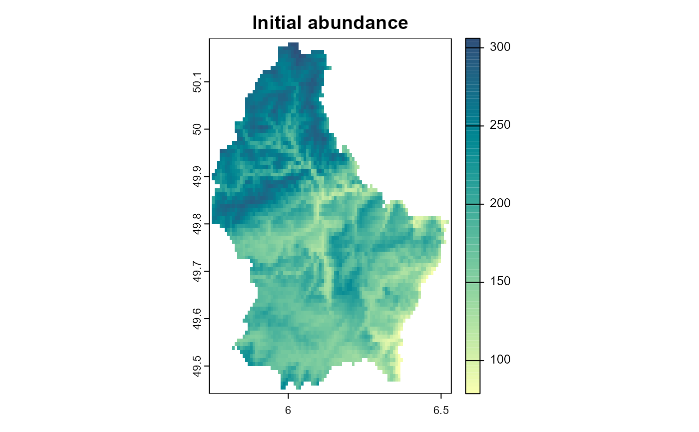
Figure 2: The initial abundance of the species.
If we would want to add a trait to all species in the simulation,
without having to type their names, we could use the already mentioned
species_names() method to get a vector of all species names
and then use that as the species argument.
sim$add_traits(
    species = sim$species_names(),
    population_level = TRUE,
    reproduction_rate = 1.5,
    carrying_capacity = 1000,
    allee_threshold = 150
)
Since we only have the two species in the simulation this
species = sim$species_names() would be equivalent to the
previous call species = c("species_1", "species_2").
Adding processes
Until now, we have two species in the simulation that are virtually identical (besides their name). If we want them to behave differently, we need add different processes to them. For the sake of this tutorial, we’ll assume that the species differ in their reproduction model.
Reproduction
Species 1 will use the same ricker_reproduction_model
from the previous vignette, with the difference that now the habitat
quality will influence the carrying capacity (i.e. we multiply the two,
before passing it to the function as input).
sim$add_process(
    species = "species_1",
    process_name = "reproduction",
    process_fun = function() {
        ricker_reproduction_model(
            self$traits$abundance,
            self$traits$reproduction_rate,
            self$traits$carrying_capacity * self$sim$environment$current$habitat_quality
        )
        print(
            paste0(self$name, " mean abundance: ", mean(self$traits$abundance))
        )
    },
    execution_priority = 1
)
In the case of species 2, we will use a Ricker model with additional
Allee effects (via the function:
ricker_allee_reproduction_model), which is an adapted
version from the model described in: Cabral, J.S. and Schurr, F.M.
(2010) [Ref. 1].
The Allee effect is also known as “depensation” or “negative density dependence” and describes multiple different mechanisms that all lead to lower reproduction rates in small populations (making them non-viable in the long term and leading to their extinction over time). Some example mechanisms of the Allee effect are: difficulties finding a mate due to low population density, or increased predation pressure due to missing protection from the crowd (see: Liermann and Hilborn, 2001) [Ref. 2].
sim$add_process(
    species = "species_2",
    process_name = "reproduction",
    process_fun = function() {
        self$traits$abundance <-
            ricker_allee_reproduction_model(
                self$traits$abundance,
                self$traits$reproduction_rate,
                self$traits$carrying_capacity * self$sim$environment$current$habitat_quality,
                self$traits$allee_threshold
            )
        print(
            paste0(self$name, " mean abundance: ", mean(self$traits$abundance))
        )
    },
    execution_priority = 1
)
Executing the simulation
Now we can execute the simulation and compare the abundance distributions of the two species.
set_verbosity(0)
sim$begin()
#> [1] "species_1 mean abundance: 348.709489547274"
#> [1] "species_2 mean abundance: 113.066829172314"
#> [1] "species_1 mean abundance: 577.208810253916"
#> [1] "species_2 mean abundance: 125.016153630418"
#> [1] "species_1 mean abundance: 497.450380346053"
#> [1] "species_2 mean abundance: 143.677696198853"
#> [1] "species_1 mean abundance: 538.40186195848"
#> [1] "species_2 mean abundance: 174.359283926975"
#> [1] "species_1 mean abundance: 518.397874403992"
#> [1] "species_2 mean abundance: 226.71976346029"
#> [1] "species_1 mean abundance: 528.487508675932"
#> [1] "species_2 mean abundance: 310.122736448007"
#> [1] "species_1 mean abundance: 523.467949256324"
#> [1] "species_2 mean abundance: 391.190632359679"
#> [1] "species_1 mean abundance: 525.983603165407"
#> [1] "species_2 mean abundance: 422.940404661898"
#> [1] "species_1 mean abundance: 524.727298281258"
#> [1] "species_2 mean abundance: 451.072431872118"
#> [1] "species_1 mean abundance: 525.355824461575"
#> [1] "species_2 mean abundance: 458.686829593375"
plot(
    sim,
    obj = "species_1",
    name = "abundance",
    main = "Species 1: abundance",
    col = plot_cols
)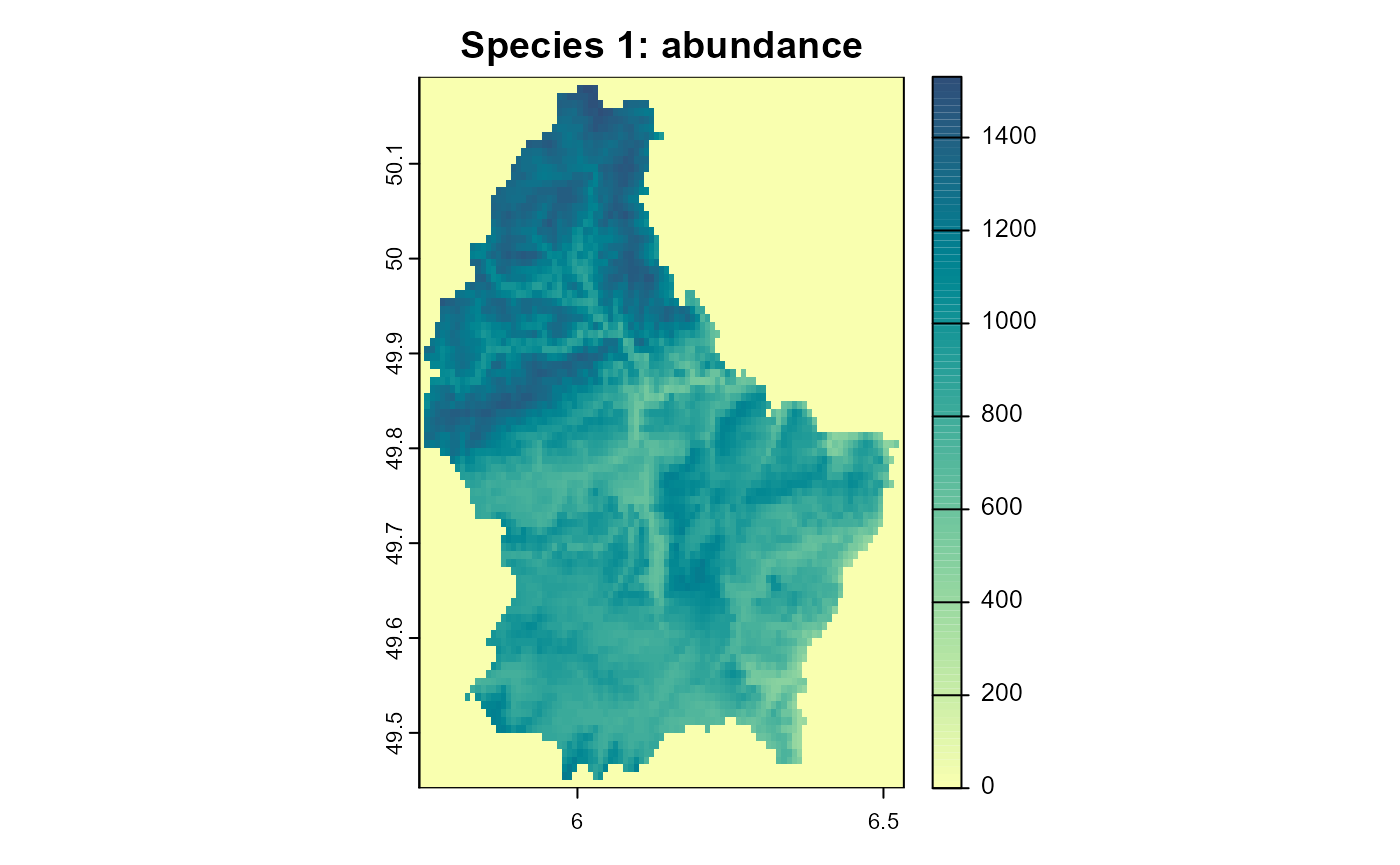
Figure 3: The resulting abundance distribution of species 1 after 10 simulation time steps.
plot(
    sim,
    obj = "species_2",
    name = "abundance",
    main = "Species 2: abundance",
    col = plot_cols
)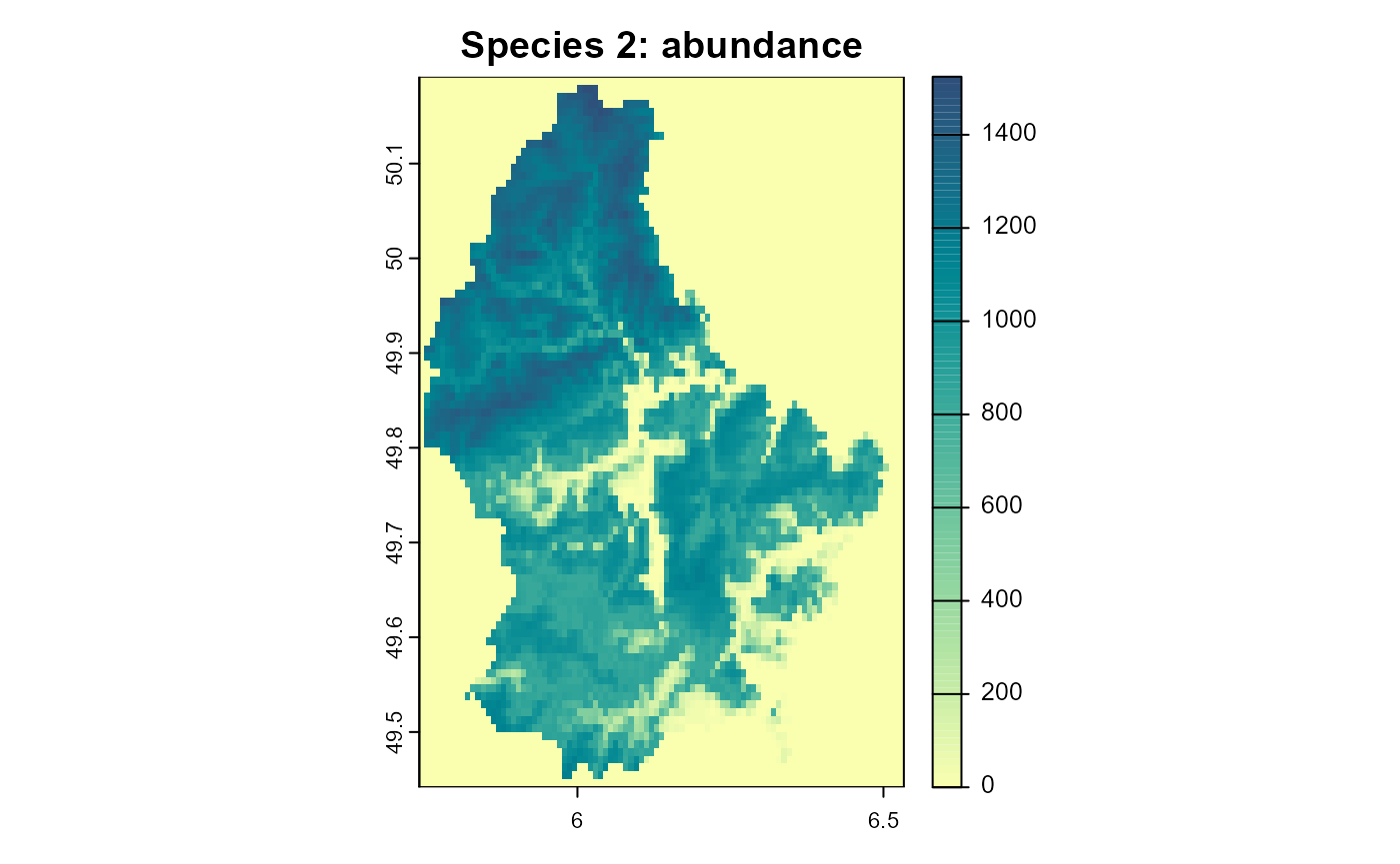
Figure 4: The resulting abundance distribution of species 2 after 10 simulation time steps.
Note how in areas of lower habitat quality, the populations of species 2 are extinct since their abundance was lower than the Allee threshold. If we would combine this with a dispersal process, this could lead to areas that are colonized by species 2, but are permanent population “sinks” for the species, since they would depend on immigration from other areas and are not self-sustaining.
References:
Cabral, J.S. and Schurr, F.M. (2010) Estimating demographic models for the range dynamics of plant species. Global Ecology and Biogeography, 19, 85–97. doi:10.1111/j.1466-8238.2009.00492.x
Liermann, and Hilborn, (2001), Depensation: evidence, models and implications. Fish and Fisheries, 2: 33–58. doi:10.1046/j.1467-2979.2001.00029.x