Niche Suitability
One of the main study question in ecology is the relationship between environmental conditions and species occurence. This tutorial will show how we can use information about the target species (e.g. preferred temperature and thermal limits) to implement a habitat suitability model in metaRange.
In a second step, we will use the calculated habitat suitability to inform the reproduction rate and carrying capacity in the population model. This allows us to see which populations are viable over time without the need for an arbitrary “suitability cutoff” value. For this, we will create a landscape with two environmental variables (temperature and precipitation) and then add two similar species to it that only differ in their environmental preferences.
At the end we can run the simulation and compare how this difference affects the distribution of the species.
We create the example landscape by arbitrarily scaling the example raster to ranges that are natural for both temperature and precipitation.
library(metaRange)library(terra)set_verbosity(2)
# find the example raster fileraster_file <- system.file("ex/elev.tif", package = "terra")
# load itr <- rast(raster_file)
# adjust the valuestemperature <- scale(r, center = FALSE, scale = TRUE) * 10 + 273.15precipitation <- r * 2terra::plot( temperature, col = hcl.colors(100, "RdYlBu", rev = TRUE), main = "Temperature [K]")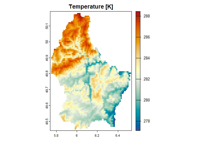
terra::plot( precipitation, col = hcl.colors(100, "Earth"), main = "Precipitation [mm]")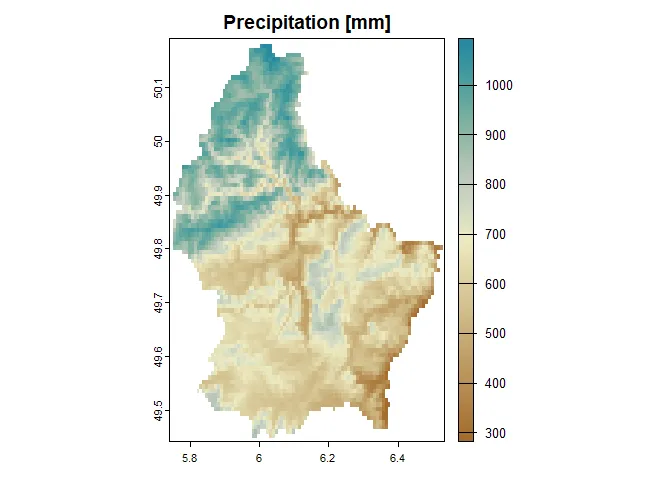
Creating the simulation and species
Section titled “Creating the simulation and species”In the previous tutorial we always created an SDS as input that has the
same number of layers as the simulation time steps. This was mainly done
to highlight the concept that one layer in the SDS represents the
conditions in one time step. In the case where the evironment is static
and does not change over time, this process is a bit tedious and also
might occupy more memory than necessary. Because of that, metaRange
provides the method set_time_layer_mapping(), which allows us to just
tell the simulation “use this one layer for every time step”. This means
we can just create an SDS that has only one layer:
landscape <- sds(temperature, precipitation)names(landscape) <- c("temperature", "precipitation")# how many layer are in the sds:terra::nlyr(landscape)#> [1] 1 1Create the simulation:
sim <- create_simulation( source_environment = landscape, ID = "example_simulation", seed = 1)#> number of time steps: 1#> time step layer mapping: 1#> added environment#> class : SpatRasterDataset#> subdatasets : 2#> dimensions : 90, 95 (nrow, ncol)#> nlyr : 1, 1#> resolution : 0.008333333, 0.008333333 (x, y)#> extent : 5.741667, 6.533333, 49.44167, 50.19167 (xmin, xmax, ymin, ymax)#> coord. ref. : lon/lat WGS 84 (EPSG:4326)#> source(s) : memory#> names : temperature, precipitation#>#> created simulation: example_simulationAnd then adjust the number of time steps and the layer that are used each time step, by calling:
# use layer 1 for 10 time stepssim$set_time_layer_mapping(rep_len(1, 10))#> number of time steps: 10#> time step layer mapping: 1, 1, 1, 1, 1, 1, 1, 1, 1, 1Now we can continue by adding the species.
sim$add_species(name = "species_1")#> adding species#> name: species_1sim$add_species(name = "species_2")#> adding species#> name: species_2Adding traits to species
Section titled “Adding traits to species”Additionally to the traits introduced in the previous tutorials we now
also add a trait called climate_suitability, where we will store the
information about how suitable the climate conditions are in each cell
for the population that lives there.
sim$add_traits( species = c("species_1", "species_2"), population_level = TRUE, abundance = 500, climate_suitability = 1, reproduction_rate = 0.3, carrying_capacity = 1000)#> adding traits:#> [1] "abundance" "climate_suitability" "reproduction_rate"#> [4] "carrying_capacity"#>#> to species:#> [1] "species_1" "species_2"#>The traits in the above example are clearly traits that need to be
stored for each population (i.e. they need to be spatially explicit).
Contrary to that, some traits may not require to be stored at the
population level. In this example, we assume that the environmental
preferences of a species are the same for all populations. This means
that when we add these traits, we can set the parameter
population_level to FALSE so that the traits are added as they are,
without expanding them to the extent of the landscape.
As mentioned in the introduction paragraph, we will give both species different environmental preferences for the two environmental variables in the simulation environment (temperature & precipitation).
Note that the names of the traits are arbitrary and can be chosen by the user and that there is no predetermined connection between e.g. “min_temperature” and the temperature variable in the environment. To establish these connections, the user needs to add processes to the species that access the correct traits and use them in a sensible way (This is why meaningful trait names are important).
sim$add_traits( species = "species_1", population_level = FALSE, max_temperature = 300, # Kelvin optimal_temperature = 288, # Kelvin min_temperature = 280, # Kelvin max_precipitation = 1000, # mm optimal_precipitation = 700, # mm min_precipitation = 200 # mm)#> adding traits:#> [1] "max_temperature" "optimal_temperature" "min_temperature"#> [4] "max_precipitation" "optimal_precipitation" "min_precipitation"#>#> to species:#> [1] "species_1"#>sim$add_traits( species = "species_2", population_level = FALSE, max_temperature = 290, optimal_temperature = 285, min_temperature = 270, max_precipitation = 1000, optimal_precipitation = 500, min_precipitation = 0)#> adding traits:#> [1] "max_temperature" "optimal_temperature" "min_temperature"#> [4] "max_precipitation" "optimal_precipitation" "min_precipitation"#> to species:#> [1] "species_2"#>Adding processes
Section titled “Adding processes”Calculate the suitability
Section titled “Calculate the suitability”To calculate the suitability, we use the metaRange function
calculate_suitability() that is based on an equation published by Yin
et al. in 1995 [Ref. 1] and simplified by Yan and Hunt in 1999 [eq:4
in Ref. 2]. The function takes the three cardinal values of an
environmental niche (minimum tolerable value, optimal vale and maximum
tolerable value) and constructs a suitability curve based on a beta
distribution.
min_value <- 270opt_value <- 285max_value <- 290x <- seq(min_value, max_value, length.out = 100)y <- calculate_suitability(max_value, opt_value, min_value, x)plot(x, y, type = "l", xlab = "Temperature [K]", ylab = "Suitability")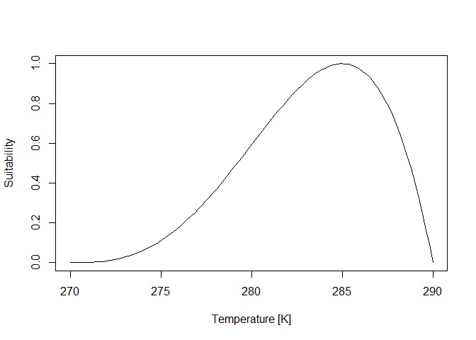
In the following code we add a process to both species that calculates the suitability for precipitation and temperature and then multiplies the values to create a joint suitability over the two environmental niches. Note that one could also define a custom function to calculate the suitability, if this built-in function does not adequately describe the ecology of the target species.
Suitability
Section titled “Suitability”sim$add_process( species = c("species_1", "species_2"), process_name = "calculate_suitability", process_fun = function() { self$traits$climate_suitability <- calculate_suitability( self$traits$max_temperature, self$traits$optimal_temperature, self$traits$min_temperature, self$sim$environment$current$temperature ) * calculate_suitability( self$traits$max_precipitation, self$traits$optimal_precipitation, self$traits$min_precipitation, self$sim$environment$current$precipitation ) }, execution_priority = 1)#> adding process: calculate_suitability#> to species:#> [1] "species_1" "species_2"#>Reproduction
Section titled “Reproduction”As in the previous tutorials, we use a Ricker reproduction model to calculate the new abundance of the species, but this time we let both the carrying capacity and the reproduction rate (for each species and population) depend on the suitability of the local environment / habitat.
sim$add_process( species = c("species_1", "species_2"), process_name = "reproduction", process_fun = function() { self$traits$abundance <- ricker_reproduction_model( self$traits$abundance, self$traits$reproduction_rate * self$traits$climate_suitability, self$traits$carrying_capacity * self$traits$climate_suitability ) }, execution_priority = 2)#> adding process: reproduction#> to species:#> [1] "species_1" "species_2"#>Results
Section titled “Results”Now, we can execute the simulation and compare the results.
set_verbosity(1)sim$begin()#> Starting simulation.#> start of time step: 1#> 10 % done | 0.017 secs remaining (estimate)#> start of time step: 2#> 20 % done | 0.018 secs remaining (estimate)#> start of time step: 3#> 30 % done | 0.018 secs remaining (estimate)#> start of time step: 4#> 40 % done | 0.033 secs remaining (estimate)#> start of time step: 5#> 50 % done | 0.011 secs remaining (estimate)#> start of time step: 6#> 60 % done | 0.0077 secs remaining (estimate)#> start of time step: 7#> 70 % done | 0.0055 secs remaining (estimate)#> start of time step: 8#> 80 % done | 0.0044 secs remaining (estimate)#> start of time step: 9#> 90 % done | 0.0022 secs remaining (estimate)#> start of time step: 10#> 100 % done | 0 secs remaining (estimate)#>#> Simulation: 'example_simulation' finished#> Exiting the Simulation#> Runtime: 0.041 secs# define a nice color paletteplot_cols <- hcl.colors(100, "Purple-Yellow", rev = TRUE)plot( sim, obj = "species_1", name = "abundance", main = "Species 1: abundance", col = plot_cols)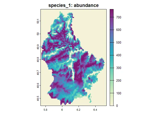
plot( sim$species_2, trait = "abundance", main = "Species 2: abundance", col = plot_cols)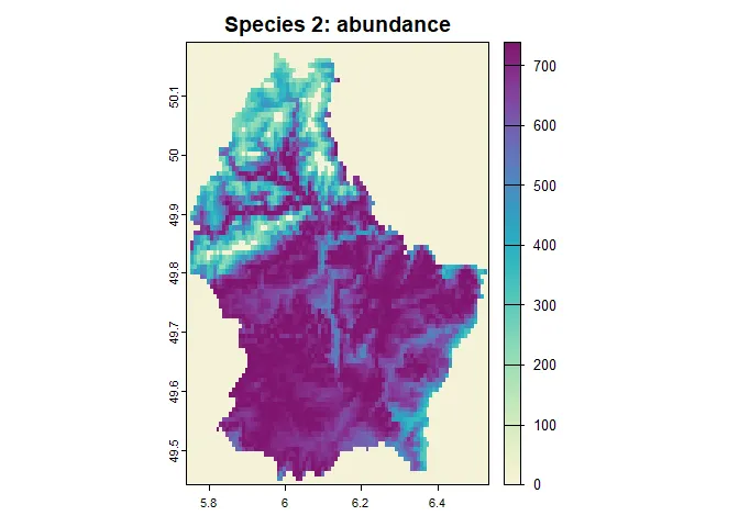
References
Section titled “References”-
Yin, X., Kropff, M.J., McLaren, G., Visperas, R.M., (1995) A nonlinear model for crop development as a function of temperature, Agricultural and Forest Meteorology, Volume 77, Issues 1-2, Pages 1–16, doi:10.1016/0168-1923(95)02236-Q
-
Yan, W., Hunt, L.A. (1999) An Equation for Modelling the Temperature Response of Plants using only the Cardinal Temperatures, Annals of Botany, Volume 84, Issue 5, Pages 607–614, ISSN 0305-7364, doi:10.1006/anbo.1999.0955