Intro

metaRange is a framework to build a variety of different process based species distribution models that can include a (basically) arbitrary number of environmental factors, processes, species and species interactions. The common denominator for all models built with metaRange is that they are raster (i.e grid) and population based.

A metaRange simulation object contains one environment that holds and manages all the environmental factors that may influence the simulation (as raster data) and one or more species that are simulated in the environment.

Each species object has two main characteristics: traits and processes. Species traits can be (somewhat arbitrary) pieces of data that describe and store information about the species while processes are functions that describe how the species interacts with itself, time, climate and other species. During each time step of the simulation, the processes of the species are executed in a user defined order and can access and modify the species traits.

While models built with metaRange can be quite variable in their structure, they are all based on population dynamics. This means that in most cases a trait will not be a single number but a matrix that has the same size as the raster data in the environment, where each value represents the trait value for one population in the corresponding grid cell of the environment. Based on this, most processes will describe population (and meta population) dynamics and not individual based mechanisms. Figure 1 shows an example of some of the different environmental factors, species traits and processes that could be included in a simulation.

Figure 1: Example of some of the different environmental factors, species traits and processes that could be included in a simulation.

A more technical overview of the different components of a simulation and how they interact with each other is shown in Figure 2. While the environment has a temporal dimension (i.e. the different time steps, see Fig.1), the traits (or the global variables of the simulation) have no temporal property. They represent the state of the species (or of the simulation respectively) in one (the current) time step. When a process is executed within a time step, it can access this current state of the simulation and modify it, which results in changing traits over the course of the simulation. Each process can be assigned a priority that is used by the process priority queue to determine in which order the processes are executed within one time step.

Figure 2: Overview of the different components of a simulation and how they interact with each other. Note that the number of species as well as the number of traits and processes per species is not limited, but only a selection is shown for simplicity.

Setting up a simulation

Following is a simple example of how to set up a simulation with metaRange, in which we only use a single species and one environmental factor (habitat quality). At the end of this introduction we will see how the abundance of the species changes in relation to the quality of the habitat each population occupies.

To start, we need to load the packages.

library(metaRange) # does the simulation
library(terra) # handles the raster data processing

Loading the landscape

The first step when setting up a simulation is the loading of the environment in which the simulation will take place. This can either be real world data or “theoretical” / generated data and may include for example different climate variables, land cover or elevation.

The simulation expects this data as an SpatRasterDataset (SDS) which is a collection of different raster files that all share the same extent and resolution. Each sub-dataset in this SDS represents one environmental variable and each layer represents one time step of the simulation. In other words, metaRange does not simulate the environmental conditions itself, but expects the user to provide the environmental data for each time step.

To create such a dataset one can use the function terra::sds(). One important note: Since each layer represents the environmental condition in one time step, all the raster files that go into the SDS need to have the same number of layers (i.e. the desired number of time steps the simulation should have). After the SDS is created, the individual sub-datasets should be named, since this is how the simulation will refer to them.

To simplify this introduction, we use an example landscape consisting only of habitat quality data, with 10 time steps (layers) that are all the same (i.e. no environmental change). Luckily the terra package has a built-in demo that we can use for this purpose.

# find the file
raster_file <- system.file("ex/elev.tif", package = "terra")

# load it
r <- rast(raster_file)

# scale it
r <- scale(r, center = FALSE, scale = TRUE)
plot(r, main = "Habitat quality")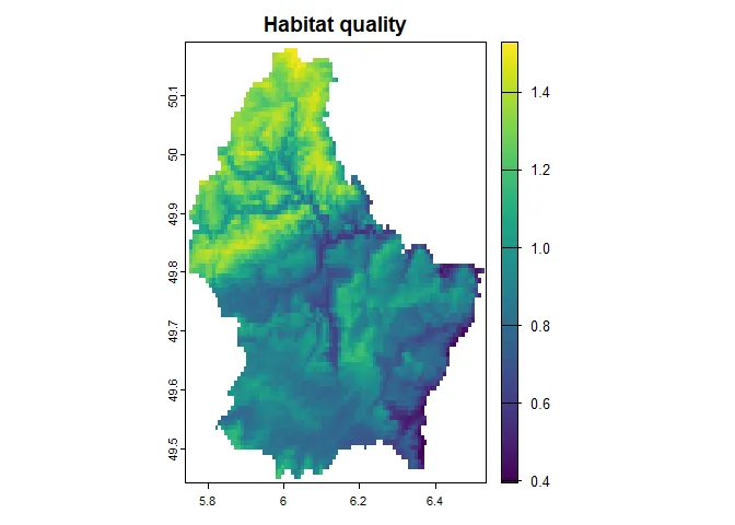

Figure 3: The habitat quality of the example landscape. Note: higher
value = better habitat
quality

Now we can turn this raster with one layer into an SDS that has multiple layer (one for each time step).

r <- rep(r, 10)
landscape <- sds(r)
names(landscape) <- c("habitat_quality")
landscape
#> class       : SpatRasterDataset
#> subdatasets : 1
#> dimensions  : 90, 95 (nrow, ncol)
#> nlyr        : 10
#> resolution  : 0.008333333, 0.008333333  (x, y)
#> extent      : 5.741667, 6.533333, 49.44167, 50.19167  (xmin, xmax, ymin, ymax)
#> coord. ref. : lon/lat WGS 84 (EPSG:4326)
#> source(s)   : memory
#> names       : habitat_quality

Pre-setup

Before creating the simulation, it may be helpful to enable extensive reporting, which will print out a lot of information each time a metaRange function is called. This can be enabled or disabled at any time (i.e. also while the simulation is running), but in order to highlight what each function call in this tutorial does, we enable it at the beginning of the setup.

# 0 = no reporting
# 1 = a bit of info
# 2 = very verbose
set_verbosity(2)

Creating the simulation

After the landscape is loaded, the simulation can be created using the create_simulation() function. The only required argument is source_environment which is the landscape / environment SDS that was created in the first step. One can optionally specify an ID for the simulation and a seed for the random number generator.

sim <- create_simulation(
    source_environment = landscape,
    ID = "example_simulation",
    seed = 1
)
#> number of time steps: 10
#> time step layer mapping: 1, 2, 3, 4, 5, 6, 7, 8, 9, 10
#> added environment
#> class       : SpatRasterDataset
#> subdatasets : 1
#> dimensions  : 90, 95 (nrow, ncol)
#> nlyr        : 10
#> resolution  : 0.008333333, 0.008333333  (x, y)
#> extent      : 5.741667, 6.533333, 49.44167, 50.19167  (xmin, xmax, ymin, ymax)
#> coord. ref. : lon/lat WGS 84 (EPSG:4326)
#> source(s)   : memory
#> names       : habitat_quality
#>
#> created simulation: example_simulation

If you want to inspect the simulation object, you can either print it, to lists its fields and methods or use the summary() function to get an overview of the simulation state.

sim
#> metaRangeSimulation object
#> Fields:
#>   $ID
#>   $globals
#>   $environment
#>   $queue
#>   $processes
#>   $seed
#> Species: none
#> Methods:
#>   $species_names()
#>   $add_globals()
#>   $add_species()
#>   $add_traits()
#>   $add_process()
#>   $begin()
#>   $exit()
#>   $set_time_layer_mapping()
#>   $get_time_layer_mapping()
#>   $get_current_time_step()
#>   $get_number_of_time_steps()
#>   $print()
#>   $summary()
summary(sim)
#> ID: example_simulation
#> Environment:
#> Fields:
#> $current ==== the environment at the current time step
#> classes     : all -> matrix
#> number      : 1
#> names       : habitat_quality
#> $sourceSDS == the source raster data of the environment
#> class       : SpatRasterDataset
#> subdatasets : 1
#> dimensions  : 90, 95 (nrow, ncol)
#> nlyr        : 10
#> resolution  : 0.008333333, 0.008333333  (x, y)
#> extent      : 5.741667, 6.533333, 49.44167, 50.19167  (xmin, xmax, ymin, ymax)
#> coord. ref. : lon/lat WGS 84 (EPSG:4326)
#> source(s)   : memory
#> names       : habitat_quality
#> Time step layer mapping:  1 2 3 4 5 6 7 8 9 10
#> Current time step:  1
#> Seed:  1
#> Species: 0
#>
#> Simulation level processes:
#> NULL
#> Gobal variables:
#> NULL
#> Queue:
#> Remaining queue (this time step):  0
#>  NULL
#> Future queue (next time step):  0
#>  NULL

Adding species to the simulation

Once the simulation is created, we can add species to it using the add_species() function. At this point we have to switch to the syntax of the R6 package that metaRange uses. This means that add_species() is a method of the simulation object and can be called using the $ operator (i.e. by indexing the simulation object and calling a function that is stored inside of it). The only required argument is names which is the name(s) of the species that will be added.

sim$add_species("species_1")
#> adding species
#> name: species_1

This species can now be accessed by using the $ operator again.

sim$species_1
#> Species:  species_1
#> processes:
#> NULL
#> traits:
#> character(0)

Adding traits to species

To assign traits to a species we can use use the add_traits() method. The first argument is species which is a character vector of species names that are already in the simulation, to which the trait should be assigned to. The second argument is population_level, a TRUE/FALSE value, that decides if the trait should be stored with one value per population (i.e. as a matrix of the same size as the landscape) or not (i.e. only one value per species). All following arguments can be supplied in the form of trait_name = trait_value.

For now we only add three traits: abundance (number of individuals in each population), reproduction_rate (how fast the populations can reproduce) and carrying_capacity (maximum number of individuals per grid cell). Note: Traits always represent the “current” state of a species. This means that the abundance we use as input here represents the initial state of the simulation. Over the course of the simulation (i.e. in each time step) the traits can be updated and changed. In this example, the abundance will change each time step while e.g. the reproduction rate stays the same, but in other cases each trait might change with time.

sim$add_traits(
    species = "species_1",
    population_level = TRUE,
    abundance = 100,
    reproduction_rate = 0.5,
    carrying_capacity = 1000
    # ...
    # Note that here could be more traits, there is no limit
)
#> adding traits:
#> [1] "abundance"         "reproduction_rate" "carrying_capacity"
#>
#> to species:
#> [1] "species_1"
#>

We can check what traits a species has by printing them:

sim$species_1$traits
#> abundance :  num [1:90, 1:95] 100 100 100 100 100 100 100 100 100 100 ...
#> carrying_capacity :  num [1:90, 1:95] 1000 1000 1000 1000 1000 1000 1000 1000 1000 1000 ...
#> reproduction_rate :  num [1:90, 1:95] 0.5 0.5 0.5 0.5 0.5 0.5 0.5 0.5 0.5 0.5 ...

Or plotting them:

plot(sim$species_1, "abundance")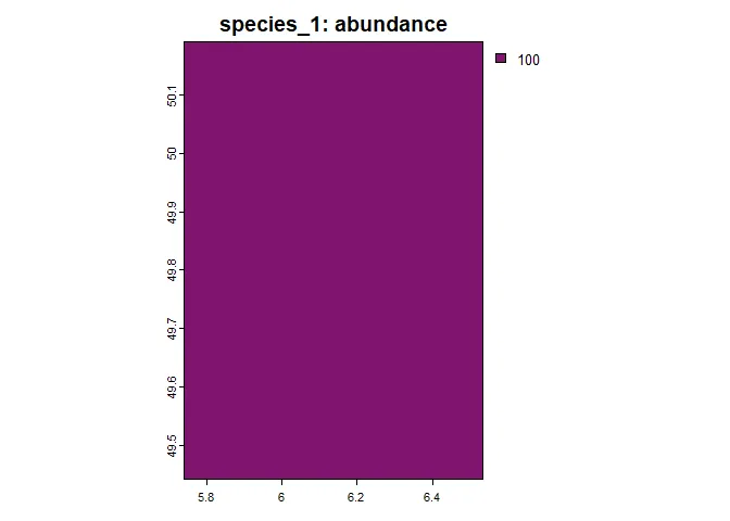

Figure 4: The initial abundance of the
species.

Note that the above plot is not very interesting, since the abundance is the same for each population at the beginning of the simulation.

Adding processes

After the species and its traits are added, the processes that describe how the species interacts with its environment can be added, using the add_process() method. The arguments are: species which is again a character vector of the species (names) that should receive the process, process_name which is a human readable name for the process and process_fun which is the function that will be called when the process is executed.

One argument that might be confusing is the execution_priority. This is a number that gives the process a priority “weight” and decides in which order the processes are executed within one time step. The smaller the number, the earlier the process will be executed (e.g. 1 gets executed before 2). In the case two (or more) processes have the same priority, it is assumed that they are independent from each other and that their execution order does not matter.

Reproduction

In this example we will only add a single process (reproduction) to the species, that is going to calculate the abundance (for each population) in the next time step, depending on the habitat quality. To do so, we can use a built-in function ricker_reproduction_model() that implements the “classic” Ricker reproduction model (Ricker, W.E. (1954)) [Ref. 1], which describes the population dynamics of a species with non-overlapping generations in discrete time steps. This model features density dependent growth and possibly also overcompensatory dynamics (i.e. the populations can, if they have a high the reproduction rate, become larger than the carrying capacity, which then leads to a decline in the next time step).

Note the use of the self keyword in the function. In this context, self refers to the species that the process is attached to. This means that the function can access the species traits and modify them and also access the environment (each species holds a reference to the simulation it was created in).

sim$add_process(
    species = "species_1",
    process_name = "reproduction",
    process_fun = function() {
        # use a ricker reproduction model
        # to calculate the new abundance
        # and let the carrying capacity
        # depend on the habitat quality
        ricker_reproduction_model(
            self$traits$abundance,
            self$traits$reproduction_rate,
            self$traits$carrying_capacity * self$sim$environment$current$habitat_quality
        )

        # print out the current mean abundance
        print(
            paste0("mean abundance: ", mean(self$traits$abundance))
        )
    },
    execution_priority = 1
)
#> adding process: reproduction
#> to species:
#> [1] "species_1"
#>

Executing the simulation

After the species, traits and processes are added to the simulation, it can be executed via the begin() method.

sim$begin()
#> Starting simulation.
#> passed initial sanity checks.
#> start of time step: 1
#> |- species_1 : reproduction
#> [1] "mean abundance: 84.1732579542268"
#> |---- 0.00082 secs
#>  10 % done | 0.012 secs remaining (estimate)
#> start of time step: 2
#> |- species_1 : reproduction
#> [1] "mean abundance: 127.598064388471"
#> |---- 0.0012 secs
#>  20 % done | 0.065 secs remaining (estimate)
#> start of time step: 3
#> |- species_1 : reproduction
#> [1] "mean abundance: 185.433176212344"
#> |---- 0.00092 secs
#>  30 % done | 0.049 secs remaining (estimate)
#> start of time step: 4
#> |- species_1 : reproduction
#> [1] "mean abundance: 254.974925085775"
#> |---- 0.00091 secs
#>  40 % done | 0.045 secs remaining (estimate)
#> start of time step: 5
#> |- species_1 : reproduction
#> [1] "mean abundance: 328.335965177599"
#> |---- 0.0015 secs
#>  50 % done | 0.039 secs remaining (estimate)
#> start of time step: 6
#> |- species_1 : reproduction
#> [1] "mean abundance: 394.79908318955"
#> |---- 8e-04 secs
#>  60 % done | 0.027 secs remaining (estimate)
#> start of time step: 7
#> |- species_1 : reproduction
#> [1] "mean abundance: 446.224976588256"
#> |---- 0.00094 secs
#>  70 % done | 0.024 secs remaining (estimate)
#> start of time step: 8
#> |- species_1 : reproduction
#> [1] "mean abundance: 480.705159122178"
#> |---- 9e-04 secs
#>  80 % done | 0.022 secs remaining (estimate)
#> start of time step: 9
#> |- species_1 : reproduction
#> [1] "mean abundance: 501.356439544315"
#> |---- 7e-04 secs
#>  90 % done | 0.006 secs remaining (estimate)
#> start of time step: 10
#> |- species_1 : reproduction
#> [1] "mean abundance: 512.803082103058"
#> |---- 0.00088 secs
#> 100 % done | 0 secs remaining (estimate)
#>
#> Simulation: 'example_simulation' finished
#> Exiting the Simulation
#> Runtime: 0.08 secs

Plotting the results

To investigate the results visually, you can just use plot().

# define a nice color palette
plot_cols <- hcl.colors(100, "BluYl", rev = TRUE)
plot(
    sim,
    obj = "species_1", # name of the species
    name = "abundance", # name of the trait to plot
    main = "Species 1: abundance", # optional title
    col = plot_cols # color palette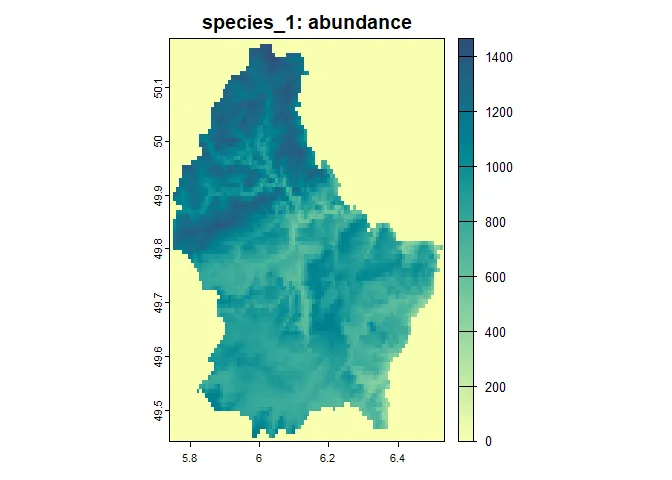
)

Figure 5: The resulting abundance distribution of species 1 after 10
simulation time
steps.

Saving the simulation

If you want to save the results (or any intermediate data) of the simulation, you can use the save_species() function. This will save the (possibly specified) traits of a species, either as a raster (.tif) or as a text (.csv) file, whatever is more appropriate for the data. Note that this function does not save the species processes. One should keep a copy of the script that is used to run the simulation to make it repeatable.

save_species(
    sim$species_1,
    traits = c("name", "of", "one_or_more", "traits"),
    path = "path/to/a/folder/"
)

References

Ricker, W.E. (1954) Stock and recruitment. Journal of the Fisheries Research Board of Canada, 11, 559–623. doi:10.1139/f54-039