Gathering data

A solid data basis is the foundation for any biodiversity model. The following text will give a short intorduction on what type of data is commonly used in biodiversity models (including metaRange) and where to find, download and how to process it.

Environmental data

It may be obvious, but it is important to restate and keep in mind that different species have different requirement for their habitat. So just using a standardized data set of environmental variables to model different species may not be the approach that yields the best results.

Similar to the question of which ecological mechanisms are needed to describe the population dynamics of a species, one should equally research the question of the true ecological niche of a species and what environmental variables best capture this niche.

There are many sources for environmental data (including predictions for the future). The “best” data source depends on the study region, the required spatial and temporal resolution as well as the avilability of different variables in the dataset.

To focus on the basics, in the following example we will gather data for the insect Mantis religiosa (European mantis) in Germany.

This species prefers warm temperatures and lives on rich structured grasslands and the border between grasslands and forests, so we will focus on the environmental variables of % grassland and summer temperature.

First we need to load the required packages and set up the default path and folder structure:

library(rgbif)              # access to GBIF species occurrence data
library(geodata)            # access to global environmental datasets
library(terra)              # raster processing
library(sf)                 # vector data processing
library(tidyverse)          # general data manipulation
library(CoordinateCleaner)  # leaning occurrence coordinates
library(ggplot2)            # plotting
library(here)               # relative paths in project

tutorial_folder_name <- "download_env_data"
dir.create(file.path(here(), tutorial_folder_name))
dir.create(file.path(here(), tutorial_folder_name, "raw_data"))
dir.create(file.path(here(), tutorial_folder_name, "processed_data"))
geodata_path(here(tutorial_folder_name, "raw_data"))

We can download the outline of of Germany to exctract the exact geographic coordinates we are interrested in. For this (and the other environmental data), we will use the geodata package that offers access to a variety of global environmental datasets.

DE <- gadm(country = "DEU", level = 0, path = geodata_path())
plot(DE)
DE_extent <- ext(DE)
DE_extent
#> SpatExtent : 5.866, 15.041, 47.270, 55.056 (xmin, xmax, ymin, ymax)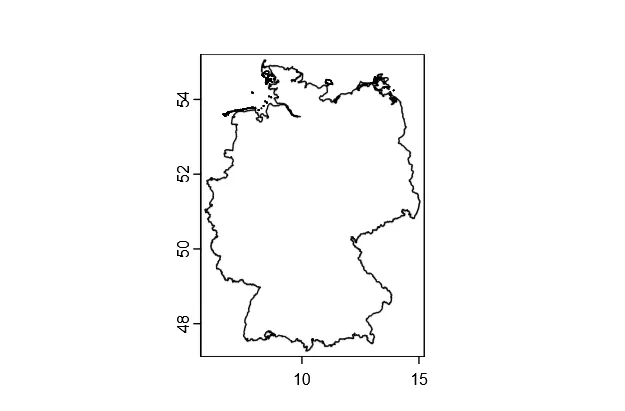

Now we can download the grassland landcover data for Germany.

DE_grassland <- landcover(var = "grassland", path = geodata_path())
DE_grassland <- crop(DE_grassland, DE_extent)
DE_grassland <- mask(DE_grassland, DE)
plot(DE_grassland, main = "% grassland")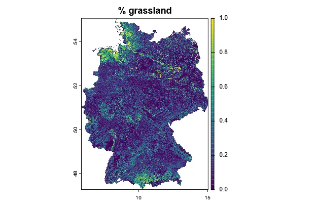

And the climate data (BIO10 = Mean Temperature of Warmest Quarter) for the reference period of 1970-2000.

DE_temp <- worldclim_country(country = "DEU", var = "bio", res = 2.5, path = geodata_path())
DE_temp <- DE_temp[["wc2.1_30s_bio_10"]]
DE_temp <- crop(DE_temp, DE_extent)
DE_temp <- mask(DE_temp, DE)
plot(DE_temp, main = "mean summer temp")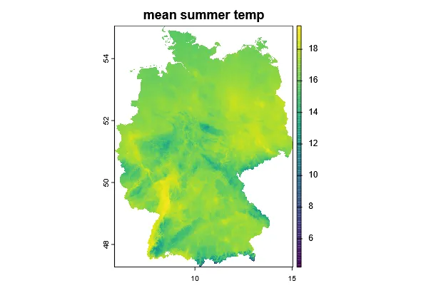

Species occurence data

For the occurence data of the species, we are goingin to download data from the Global Biodiversity Information Facility (GBIF). GBIF offers the R package rgbif that lets you search and download occurence data directly from R. There are plenty of options to construct this search query, including some to get citable DOIs for the data you download. Here, we will keep it simple and just search for occurences in Germany that have coordinates and limit the number of results to 1000.

# query and download data
occ_data <- occ_search(
    scientificName = "Mantis religiosa",
    country = "DE",
    hasCoordinate = TRUE,
    limit = 1000
)
# clean coordinates (remove common errors)
occ_data_clean <- clean_coordinates(
    x = occ_data$data,
    lon = "decimalLongitude",
    lat = "decimalLatitude",
    species = "species",
    tests = c("centroids", "equal", "gbif", "institutions", "zeros")
)
# convert to spatial vector
occurence <- vect(data.frame(
    lon = occ_data_clean$decimalLongitude,
    lat = occ_data_clean$decimalLatitude
), crs = "EPSG:4326")
# exclude points outside Germany
occurence <- crop(occurence, DE_extent)
plot(occurence)
plot(DE, add = TRUE)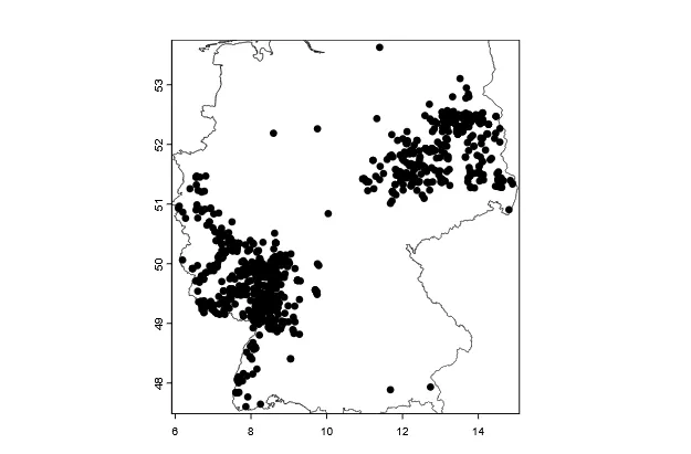

Finally, we can save the processed data to the project folder for later use.

writeVector(
    occurence,
    here(tutorial_folder_name, "processed_data", "Mantis_religiosa_occurrence.shp"),
    overwrite=TRUE)
writeRaster(
    DE_grassland, here(tutorial_folder_name,
    "processed_data", "DE_grassland.tif"),
    overwrite=TRUE)
writeRaster(
    DE_temp,
    here(tutorial_folder_name, "processed_data", "DE_bio10.tif"),
    overwrite=TRUE)

Niche estimation example

To estimate the species niche based on the gathered data, we can now extract the environmental values at the occurence points and use that data “fit” a normal distribution that can represent the species niche.

temp_extr <- terra::extract(DE_temp, occurence)
names(temp_extr)<- c("ID","temperature")
temp_extr <- temp_extr[!is.na(temp_extr$temperature), ]

Estimate the niche based on these values

temp_density <- density(temp_extr$temperature, bw = 2)
temp_max_density <- temp_density$x[which.max(temp_density$y)]
temp_min <- quantile(temp_extr$temperature, probs = 0.0025)
temp_max <- quantile(temp_extr$temperature, probs = 0.9975)

Combine the data and plot it

temp_combined <- temp_extr
temp_combined$type <- "extracted"
temp_normal <- rnorm(10000, temp_max_density, sd = abs((temp_min - temp_max)) / (6))
temp_normal <- data.frame("temperature" = temp_normal, "ID"= NA, "type" = "estimated")
temp_combined <- rbind(temp_combined, temp_normal)

temp_plot <-
  ggplot(temp_combined, aes(x=temperature, after_stat(scaled), fill=type)) +
    geom_density(color="#e9ecef", alpha=0.8) +
    ylab("scaled frequency") +
    scale_fill_manual(values=c("darkorange3", "darkred")) +
    theme_dark()
temp_plot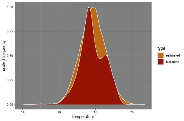

As you can see, the estimated niche (orange) fits quite well to the extracted data (red).

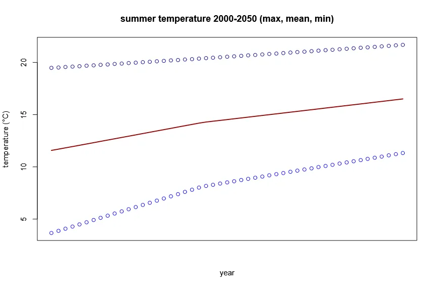
Warning: Before using this niche in a model, one should evaluate if the estimated niche makes ecologial sense and compare it to literature values. It may include biases based on the occurence data used.

Creating time series data

Many correlative species distribution models only need a singular future time step to produce predictions (e.g. the environmental data for the year 2100). Contrary, most mechanistic biodiversity models require time series data of environmental variables, because they explcitly simulate the processes that drive population dynamics in each time step. Unfortunatly, many of the climate models that produce the future scenarios only provide data for a few time steps (e.g. 2050 and 2100). Following we will show how to use a simple linear interpolation to create a continuous time series from the 2000 to 2050.

The first step is to download the future prediction for our variables of choice (BIO10 = Mean Temperature of Warmest Quarter) for our target year 2050. The geodata package also provides access to these data via the cmip6_world function. We will focus on the Shared Socio-economic Pathway (ssp) 585 and the general circulation model (gcm) “MPI-ESM1-2-HR”.

bio10_2050 <- cmip6_world(
    var = "bio",
    model = "MPI-ESM1-2-HR",
    ssp = "585",
    time = "2041-2060",
    res = 5,
    path = geodata_path()
)
# select BIO10
bio10_2050 <- bio10_2050[["bio10"]]
# resample to same resolution as current data
bio10_2050 <- resample(bio10_2050, DE_temp, method = "bilinear")
# crop and mask to Germany
bio10_2050 <- crop(bio10_2050, DE_extent)
bio10_2050 <- mask(bio10_2050, DE)

Now we can use the function approximate to interpolate between these two time steps.

temp <- rast(DE_temp)
# create empty raster with 51 layers (2000-2050)
nlyr(temp) <- 51

# assign the two known time steps
temp[[1]] <- DE_temp
temp[[51]] <- bio10_2050

# interpolate the missing years
temp <- approximate(temp, method = "linear")
temp
# class       : SpatRaster
# dimensions  : 935, 1101, 51  (nrow, ncol, nlyr)
# resolution  : 0.008333333, 0.008333333  (x, y)
# extent      : 5.866667, 15.04167, 47.26667, 55.05833  (xmin, xmax, ymin, ymax)
# coord. ref. : lon/lat WGS 84 (EPSG:4326)
# source(s)   : memory
# names       : wc2.1~io_10,     lyr.2,    lyr.3,     lyr.4,     lyr.5,    lyr.6, ...
# min values  :    3.666667,  3.873613,  4.08056,  4.287507,  4.494453,  4.70140, ...
# max values  :   19.483334, 19.521042, 19.55875, 19.596459, 19.637154, 19.67978, ...

And now just to visualize the time series:

temp_vec <- minmax(temp, compute=FALSE)
temp_min <- temp_vec[1, ]
temp_max <- temp_vec[2, ]
temp_mean <- (temp_min + temp_max) / 2
plot(temp_min,
    ylim=c(min(temp_min), max(temp_max)),
    main = "summer temperature 2000-2050 (max, mean, min)",
    type ="p", col="blue1",
    ylab="temperature (°C)", xlab="year",
    xaxt="n")
lines(temp_mean, col="darkred", lwd=2)
points(temp_max, col="blue4")